Sample-basierti Quantediagonalisiеrig vo emene Chemie-Hamiltonian

Schätzige zum Recheufwand: under eim Minüüt uf emem Heron-r2-Prozessor (ACHTUNG: Das isch nur e Schätzig. Dini Laufziit cha abwiche.)

Hintergrundinformatione

I däm Tutorial zeige mir, wie mer rüschbehafti Quantesamples nachbearbeite cha, zum e Näheriig vom Grundzuestand vom Stickstoffmolekül $\text{N}_2$ bim Gliichgewichtsbindungsabstand z'finde. Mir verwände derfür de sample-basierte Quantediagonalisierigalgorithmus (SQD) mit Samples us emem 59-Qubit-Quanteschaltkreis (52 System-Qubits + 7 Ancilla-Qubits). E Qiskit-basierti Implementierig isch i de SQD Qiskit Addons verfüegbar. Meh Details finsch i de entsprechende Docs sowie emem eifache Bispiil zum Iisteige.

SQD isch e Technik zum Finde vo Eigewärt und Eigevektore vo Quanteoperatore, wie zum Bispiil em Hamiltonian vomene Quantesystem. Derfür setzt si Quante- und verteilets klassisches Rechene zämme ii. Klassischs verteiltes Rechene wird bruucht, zum Samples vo emem Quanteprozessor z'verarbeite und emene Ziil-Hamiltonian i emem vo ihne ufgspannte Unterruum z'projiziere und diagonalisiere. Das macht SQD robust gegenüber Samples, wo vo Quanterüsche korrumpiert worde sind, und ermöglicht s'Umgah mit grosse Hamiltonians — zum Bispiil Chemie-Hamiltonians mit Millione vo Wächselwürkigstärme — witer us em Erreichbare vo jedere exakte Diagonalisierigsmethode. E SQD-basierter Workflow het folgendi Schritt:

1. Wähl e Schaltkreis-Ansatz und wänd ihn uf emem Quantecomputer uf emem Referenzzuestand aa (i däm Fall em Hartree-Fock-Zuestand).
2. Sample Bitfolge us em resultierete Quantezuestand.
3. Füehr d'selbstkonsistenti Konfigurationswiederherstellig uf de Bitfolge dür, zum d'Näheriig vomene Grundzuestand z'erhalte.

SQD funktioniert bekanntermaasse guet, wenn de Ziil-Eigezuestand dünn bsetzt isch: D'Wellefunktion isch uf eme Satz vo Basiszueständ $\mathcal{S} = \{|x\rangle \}$ gstützt, wo sini Grösse nöd exponentiell mit der Grösse vom Problem zunimmt.

Quantechemie

D'Eigenschafte vo Molekül wärde grossteils dur d'Struktur vo de Elektronen i ihne bstimmt. Als fermionischi Teilche chöi Elektronen mit emem mathematische Formalismus bschriibe wärde, wos als zwöiti Quantisierig bezeichnet wird. D'Idee isch, dass es e Azahl vo Orbitale git, wo jeweils entweder leer oder vo emem Fermion bsetzt sind. E System vo $N$ Orbitalen wird dur e Satz vo fermionische Vernichtungsoperatore $\{\hat{a}_p\}_{p=1}^N$ bschriibe, wo d'fermionische Antivertauschigrelatiône erfülle:

$$\begin{align*} \hat{a}_p \hat{a}_q + \hat{a}_q \hat{a}_p &= 0, \\ \hat{a}_p \hat{a}_q^\dagger + \hat{a}_q^\dagger \hat{a}_p &= \delta_{pq}. \end{align*}$$

Dr Adjungierte $\hat{a}_p^\dagger$ wird Erzeugungsoperator gnennt.

Bis jetzt het üseri Darstellig de Spin nöd berücksichtigt — e fundamentale Eigenschaft vo Fermione. Wenn mer de Spin mit iinimmt, chöme d'Orbitale in Paar vor, wo Raumorbitalе gnennt wärde. Jedes Raumorbital besteit us zwöi Spinorbitalen — eis mit de Bezeichnig «Spin-$\alpha$» und eis mit «Spin-$\beta$». Mir schriibe $\hat{a}_{p\sigma}$ für de Vernichtungsoperator, wo zum Spinorbital mit Spin $\sigma$ ($\sigma \in \{\alpha, \beta\}$) im Raumorbital $p$ ghört. Wenn $N$ d'Azahl vo Raumorbitale isch, git es isgsamnt $2N$ Spinorbitale. Dr Hilbert-Ruum vo däm System wird vo $2^{2N}$ orthonormierte Basisvektore ufgspannt, wo mit zweiteilige Bitfolge $\lvert z \rangle = \lvert z_\beta z_\alpha \rangle = \lvert z_{\beta, N} \cdots z_{\beta, 1} z_{\alpha, N} \cdots z_{\alpha, 1} \rangle$ bezeichnet wärde.

Dr Hamiltonian vomene Molekülsystem cha gschriibe wärde als

$$\hat{H} = \sum_{ \substack{pr\\\sigma} } h_{pr} \, \hat{a}^\dagger_{p\sigma} \hat{a}_{r\sigma} + \frac12 \sum_{ \substack{prqs\\\sigma\tau} } h_{prqs} \, \hat{a}^\dagger_{p\sigma} \hat{a}^\dagger_{q\tau} \hat{a}_{s\tau} \hat{a}_{r\sigma},$$

wo $h_{pr}$ und $h_{prqs}$ komplexe Zahle sind, wo Molekülintegrale gnennt wärde und vo de Spezifikatione vom Molekül mit emem Computerprogramm berechnet wärde chöi. I däm Tutorial berechne mir d'Integrale mit em PySCF-Softwarepaket.

Für Details derzue, wie dr molekulare Hamiltonian abgeleitet wird, lueg in es Läehrbüech über Quantechemie ine (zum Bispiil Modern Quantum Chemistry vo Szabo und Ostlund). Für e übergeordneti Erchlärig, wie Quantechemieprobleem uf Quantecomputer abgbildet wärde, lueg di d'Vorlesig Mapping Problems to Qubits vo der Qiskit Global Summer School 2024 aa.

Lokaler unitärer Cluster-Jastrow (LUCJ)-Ansatz

SQD bruucht e Quanteschaltkreis-Ansatz, um Samples drus z'ziehe. I däm Tutorial verwände mir de lokale unitäre Cluster-Jastrow (LUCJ)-Ansatz, wel er physikalisch motiviert und gliichzitig hardwarefrindlich isch.

Dr LUCJ-Ansatz isch e spezialisiertè Form vomene allgemeinen unitären Cluster-Jastrow (UCJ)-Ansatz, wo d'Form het:

$$\lvert \Psi \rangle = \prod_{\mu=1}^L e^{\hat{K}_\mu} e^{i \hat{J}_\mu} e^{-\hat{K}_\mu} | \Phi_0 \rangle$$

wo $\lvert \Phi_0 \rangle$ e Referenzzuestand isch (oft dr Hartree-Fock-Zuestand), und d'$\hat{K}_\mu$ und $\hat{J}_\mu$ d'Form hend:

$$\hat{K}_\mu = \sum_{pq, \sigma} K_{pq}^\mu \, \hat{a}^\dagger_{p \sigma} \hat{a}^{\phantom{\dagger}}_{q \sigma} \;,\; \hat{J}_\mu = \sum_{pq, \sigma\tau} J_{pq,\sigma\tau}^\mu \, \hat{n}_{p \sigma} \hat{n}_{q \tau} \;,$$

wo mir de Zahloperator definiert hend als

$$\hat{n}_{p \sigma} = \hat{a}^\dagger_{p \sigma} \hat{a}^{\phantom{\dagger}}_{p \sigma}.$$

Dr Operator $e^{\hat{K}_\mu}$ isch e Orbitalrotiig, wo sich mit bekannte Algorithme in linearer Tiifen und linearer Verbindigkeit implementiere laat. Zum Implementiere vom $e^{i \mathcal{J}_k}$-Tärm vomene UCJ-Ansatz bruucht mer entweder All-to-all-Verbindigkeite oder e fermionisches Swap-Netz, was für rüschbehafti, nöd fählertoleranti Quanteprozessore mit beschränkter Verbindigkeite schwierig isch. D'Idee vomene lokale UCJ-Ansatz isch, Dünnbsetzigsbeschränkige an d'$\mathbf{J}^{\alpha\alpha}$- und $\mathbf{J}^{\alpha\beta}$-Matrize z'lege, wo s'Implementiere in konstanter Tiifen uf Qubit-Topologiee mit beschränkter Verbindigkeite ermögliche. D'Beschränkige wärde dur e Lischt vo Indices agee, wo aaluege, welchi Matrizenträge im obere Dreick ungleich null si dörfe (da d'Matrize symmetrisch sind, muss nur s'obere Dreick aagee wärde). Die Indices chöi als Paare vo Orbitale interpretiiert wärde, wo mitänand wächselwürke dörfe.

Als Bispiil luege mir e quadratischi Gitter-Qubit-Topologie aa. Mir chöi d'$\alpha$- und $\beta$-Orbitale in parallele Linie uf em Gitter platziere, mit Verbindigkeite zwüsche dene Linie, wo «Sprossen» vomene Läitermuscht bilde, ettewää so:

Mit däm Setup sind Orbitale mit em glyche Spin mit ere Liniентопологіе verbunde, während Orbitale mit unterschiedlichem Spin verbunde sind, wenn si dasselb Raumorbital teiiled. Das git d'folgendi Indexbeschränkige für d'$\mathbf{J}$-Matrize:

$$\begin{align*} \mathbf{J}^{\alpha\alpha} &: \set{(p, p+1) \; , \; p = 0, \ldots, N-2} \\ \mathbf{J}^{\alpha\beta} &: \set{(p, p) \;, \; p = 0, \ldots, N-1} \end{align*}$$

Anders gseit: Wenn d'$\mathbf{J}$-Matrize nur an de aagäbene Indices im obere Dreick ungleich null sind, cha dr $e^{i \mathcal{J}_k}$-Tärm uf ere quadratische Topologie ohne Swap-Gates in konstanter Tiifen implementiert wärde. Natürlich macht das de Ansatz weniger ausdrucksstark, drum wärde möglicherwiis meh Ansatz-Widerholigе bruucht.

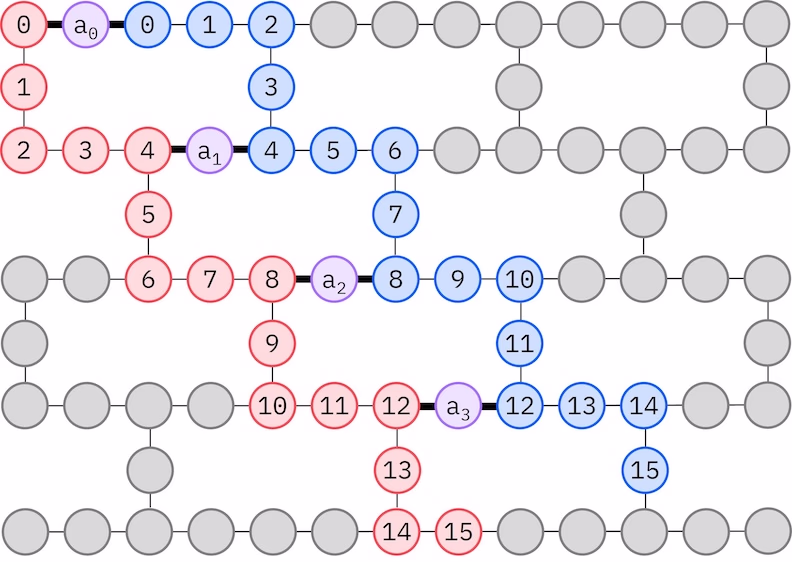
D'IBM®-Hardware het e Heavy-Hex-Gitter-Qubit-Topologie. Dert chame es «Zickzack»-Muscht verwände, wie unten dargstellt. I däm Muscht wärde Orbitale mit em glyche Spin uf Qubits mit ere Linientopologie abgbildet (roti und blaui Chraise), und e Verbindig zwüsche Orbitalen mit unterschiedlichem Spin isch bi jedem 4. Raumorbital vorhanden — ermöglicht dur e Ancilla-Qubit (violetti Chraise). In däm Fall sind d'Indexbeschränkige:

$$\begin{align*} \mathbf{J}^{\alpha\alpha} &: \set{(p, p+1) \; , \; p = 0, \ldots, N-2} \\ \mathbf{J}^{\alpha\beta} &: \set{(p, p) \;, \; p = 0, 4, 8, \ldots (p \leq N-1)} \end{align*}$$

Selbstkonsistenti Konfigurationswiederherstellig

D'selbstkonsistenti Konfigurationswiederherstellig isch drum entwicklet worde, damit mer so vill Signal wie möglich us rüschbehaftne Quantesamples herauszieht. Well dr molekulare Hamiltonian d'Teilchezahl und den Spin Z konserviert, macht's Sinn, e Schaltkreis-Ansatz z'wähle, wo au die Symmetriee konserviert. Wenn mer ihn uf em Hartree-Fock-Zuestand aawändet, het dr resultierete Zuestand im rüschfreiee Fall e fixierti Teilchezahl und nen fixierter Spin Z. Drum sötted d'Spin-$\alpha$- und Spin-$\beta$-Hälfte vo jedere Bitfolge, wo us däm Zuestand gsampled wird, dasselb Hamming-Gwicht haa wie im Hartree-Fock-Zuestand. Dur d'Prääsenz vo Rüschen in aktuelle Quanteprozessore wärde manche gmässeni Bitfolge disi Eigenschaft verlätze. E eifachi Form vo Nachauswahl würd die Bitfolge verwerfe, aber das isch verschwänderisch, denn si könnted trotzdem no Signal enthalte. D'selbstkonsistenti Wiederherstelligsvorgehenswiis versuecht, nes Teil vo däm Signal i dr Nachbearbeitig z'rette. D'Vorgehenswiis isch iterativ und bruucht als Iigab e Schätzig vo de mittlere Besetzigszahle vo jedem Orbital im Grundzuestand, wo zerscht us de rohe Samples berechnet wird. D'Vorgehenswiis wird i eme Schalter uf gfüehrt, und jedi Iteration het folgendi Schritt:

1. Für jedi Bitfolge, wo d'aagäbene Symmetriee verletzt, flip iri Bits mit emem probabilistischen Verfahre, wo d'Bitfolge nöcher zur aktuelle Schätzig vo de mittlere Orbitalbesetzige bringe soll, um e neui Bitfolge z'erhalte.
2. Sammel alli alte und neie Bitfolge, wo d'Symmetriee erfülle, und wähl Teilmängе vo nere fixiertе Grösse us, wo im Voraus bstimmt wird.
3. Für jedi Teilmängi vo Bitfolge, projizier de Hamiltonian in de Unterruum, wo vo de entsprechende Basisvektore ufgspannte wird (lueg im vorherige Abschnitt für e Beschriibig vo dene Basisvektore), und berechne uf emem klassischen Computer e Grundzuestandsschätzig vomene projizierten Hamiltonian.
4. Aktualisier d'Schätzig vo de mittlere Orbitalbesetzige mit der Grundzuestandsschätzig, wo d'tiefschti Energie het.

SQD-Workflow-Diagramm

Dr SQD-Workflow isch im folgenden Diagramm dargstellt:

Vorussetzige

Bevor du mit däm Tutorial aafangsch, sorg derfür, dass du Folgendes installiert hesch:

• Qiskit SDK v1.0 oder nöier, mit Visualisierigssupport
• Qiskit Runtime v0.22 oder nöier (pip install qiskit-ibm-runtime)
• SQD Qiskit Addon v0.11 oder nöier (pip install qiskit-addon-sqd)
• ffsim v0.0.58 oder nöier (pip install ffsim)

Setup

# Added by doQumentation — installs packages not in the Binder environment
!pip install -q ffsim qiskit-addon-sqd

import pyscf
import pyscf.cc
import pyscf.mcscf
import ffsim
import numpy as np
import matplotlib.pyplot as plt

from qiskit import QuantumCircuit, QuantumRegister
from qiskit.transpiler.preset_passmanagers import generate_preset_pass_manager

from qiskit_ibm_runtime import QiskitRuntimeService
from qiskit_ibm_runtime import SamplerV2 as Sampler

Schritt 1: Klassischi Iigabe uf es Quanteproblem abbilden

I däm Tutorial wärde mir e Näheriig zum Grundzuestand vomene Moleküls im Gliichgewicht im cc-pVDZ-Basissatz suuche. Zerscht spezifiziere mir s'Molekül und sini Eigenschafte.

# Specify molecule properties
open_shell = False
spin_sq = 0

# Build N2 molecule
mol = pyscf.gto.Mole()
mol.build(
    atom=[["N", (0, 0, 0)], ["N", (1.0, 0, 0)]],
    basis="cc-pvdz",
    symmetry="Dooh",
)

# Define active space
n_frozen = 2
active_space = range(n_frozen, mol.nao_nr())

# Get molecular integrals
scf = pyscf.scf.RHF(mol).run()
num_orbitals = len(active_space)
n_electrons = int(sum(scf.mo_occ[active_space]))
num_elec_a = (n_electrons + mol.spin) // 2
num_elec_b = (n_electrons - mol.spin) // 2
cas = pyscf.mcscf.CASCI(scf, num_orbitals, (num_elec_a, num_elec_b))
mo = cas.sort_mo(active_space, base=0)
hcore, nuclear_repulsion_energy = cas.get_h1cas(mo)
eri = pyscf.ao2mo.restore(1, cas.get_h2cas(mo), num_orbitals)

# Store reference energy from SCI calculation performed separately
exact_energy = -109.22690201485733

converged SCF energy = -108.929838385609

Bevor mir de LUCJ-Ansatz-Schaltkreis konstruiere, füehre mir zerscht e CCSD-Berechniig in der folgenden Code-Zelle dür. D'$t_1$- und $t_2$-Amplituden us dere Berechniig wärde bruucht, zum d'Parameter vomene Ansatzes z'initialisiere.

# Get CCSD t2 amplitudes for initializing the ansatz
ccsd = pyscf.cc.CCSD(
    scf, frozen=[i for i in range(mol.nao_nr()) if i not in active_space]
).run()
t1 = ccsd.t1
t2 = ccsd.t2

E(CCSD) = -109.2177884185543  E_corr = -0.2879500329450045

Jetzt verwände mir ffsim, zum de Ansatz-Schaltkreis z'erstelle. Da üses Molekül e closed-shell-Hartree-Fock-Zuestand het, verwände mir d'spin-balancierti Variante vomene UCJ-Ansatzes, UCJOpSpinBalanced. Mir übergäbe Wächselwürkigspaare, wo für e Heavy-Hex-Gitter-Qubit-Topologie passend sind (lueg im Hintergrundsabschnitt über de LUCJ-Ansatz). Mir setzend optimize=True i dr from_t_amplitudes-Methode, zum d'«komprimierti» Doppelfaktorisierig vo de $t_2$-Amplituden z'aktiviere (lueg The local unitary cluster Jastrow (LUCJ) ansatz in der ffsim-Dokumentation für Details).

n_reps = 1
alpha_alpha_indices = [(p, p + 1) for p in range(num_orbitals - 1)]
alpha_beta_indices = [(p, p) for p in range(0, num_orbitals, 4)]

ucj_op = ffsim.UCJOpSpinBalanced.from_t_amplitudes(
    t2=t2,
    t1=t1,
    n_reps=n_reps,
    interaction_pairs=(alpha_alpha_indices, alpha_beta_indices),
    # Setting optimize=True enables the "compressed" factorization
    optimize=True,
    # Limit the number of optimization iterations to prevent the code cell from running
    # too long. Removing this line may improve results.
    options=dict(maxiter=1000),
)

nelec = (num_elec_a, num_elec_b)

# create an empty quantum circuit
qubits = QuantumRegister(2 * num_orbitals, name="q")
circuit = QuantumCircuit(qubits)

# prepare Hartree-Fock state as the reference state and append it to the quantum circuit
circuit.append(ffsim.qiskit.PrepareHartreeFockJW(num_orbitals, nelec), qubits)

# apply the UCJ operator to the reference state
circuit.append(ffsim.qiskit.UCJOpSpinBalancedJW(ucj_op), qubits)
circuit.measure_all()

Schritt 2: Problem für d'Quantehardware-Uusfüehrig optimiere

Als nöchschts optimiere mir de Schaltkreis für e Ziil-Hardware.

service = QiskitRuntimeService()
backend = service.least_busy(
    operational=True, simulator=False, min_num_qubits=133
)

print(f"Using backend {backend.name}")

Using backend ibm_fez

Mir empfähle folgendi Schritt zum Optimiere vomene Ansatzes und zum Hardware-kompatibel Mache:

• Wähl physikalisch Qubits (initial_layout) vo der Ziil-Hardware us, wo dem vorher bschriibene «Zickzack»-Muscht entspreche. S'Aalege vo Qubits in däm Muscht führt zu emem effiziente hardwarekompatible Schaltkreis mit weniger Gates. Hie isch Kod, wo d'Uuswahl vomene «Zickzack»-Muschts automatisiert und e Scoring-Heuristik bruchт, um d'Fähler bi em gwählte Layout z'minimiere.
• Generier e gestuften Passmanger mit der generate_preset_pass_manager-Funktion vo Qiskit mit dim backend und dimem initial_layout.
• Setz d'pre_init-Schtuf vo dimem gestuften Passmanager uf ffsim.qiskit.PRE_INIT. ffsim.qiskit.PRE_INIT enthält Qiskit-Transpiler-Päss, wo Gates in Orbitalrotiigene zerläge und dann d'Orbitalrotiigene zämmefüehre, was zu weniger Gates im Endschaltkreis führt.
• Füehr de Passmanager uf dimem Schaltkreis us.

Kod für d'automatisierti Uuswahl vomene «Zickzack»-Layouts

from typing import Sequence

import rustworkx
from qiskit.providers import BackendV2
from rustworkx import NoEdgeBetweenNodes, PyGraph

IBM_TWO_Q_GATES = {"cx", "ecr", "cz"}

def create_linear_chains(num_orbitals: int) -> PyGraph:
    """In zig-zag layout, there are two linear chains (with connecting qubits between
    the chains). This function creates those two linear chains: a rustworkx PyGraph
    with two disconnected linear chains. Each chain contains `num_orbitals` number
    of nodes, that is, in the final graph there are `2 * num_orbitals` number of nodes.

    Args:
        num_orbitals (int): Number orbitals or nodes in each linear chain. They are
            also known as alpha-alpha interaction qubits.

    Returns:
        A rustworkx.PyGraph with two disconnected linear chains each with `num_orbitals`
            number of nodes.
    """
    G = rustworkx.PyGraph()

    for n in range(num_orbitals):
        G.add_node(n)

    for n in range(num_orbitals - 1):
        G.add_edge(n, n + 1, None)

    for n in range(num_orbitals, 2 * num_orbitals):
        G.add_node(n)

    for n in range(num_orbitals, 2 * num_orbitals - 1):
        G.add_edge(n, n + 1, None)

    return G

def create_lucj_zigzag_layout(
    num_orbitals: int, backend_coupling_graph: PyGraph
) -> tuple[PyGraph, int]:
    """This function creates the complete zigzag graph that 'can be mapped' to an IBM QPU with
    heavy-hex connectivity (the zigzag must be an isomorphic sub-graph to the QPU/backend
    coupling graph for it to be mapped).
    The zigzag pattern includes both linear chains (alpha-alpha interactions) and connecting
    qubits between the linear chains (alpha-beta interactions).

    Args:
        num_orbitals (int): Number of orbitals, that is, number of nodes in each alpha-alpha linear chain.
        backend_coupling_graph (PyGraph): The coupling graph of the backend on which the LUCJ ansatz
            will be mapped and run. This function takes the coupling graph as a undirected
            `rustworkx.PyGraph` where there is only one 'undirected' edge between two nodes,
            that is, qubits. Usually, the coupling graph of a IBM backend is directed (for example, Eagle devices
            such as ibm_brisbane) or may have two edges between two nodes (for example, Heron `ibm_torino`).
            A user needs to be make such graphs undirected and/or remove duplicate edges to make them
            compatible with this function.

    Returns:
        G_new (PyGraph): The graph with IBM backend compliant zigzag pattern.
        num_alpha_beta_qubits (int): Number of connecting qubits between the linear chains
            in the zigzag pattern. While we want as many connecting (alpha-beta) qubits between
            the linear (alpha-alpha) chains, we cannot accommodate all due to qubit and connectivity
            constraints of backends. This is the maximum number of connecting qubits the zigzag pattern
            can have while being backend compliant (that is, isomorphic to backend coupling graph).
    """
    isomorphic = False
    G = create_linear_chains(num_orbitals=num_orbitals)

    num_iters = num_orbitals
    while not isomorphic:
        G_new = G.copy()
        num_alpha_beta_qubits = 0
        for n in range(num_iters):
            if n % 4 == 0:
                new_node = 2 * num_orbitals + num_alpha_beta_qubits
                G_new.add_node(new_node)
                G_new.add_edge(n, new_node, None)
                G_new.add_edge(new_node, n + num_orbitals, None)
                num_alpha_beta_qubits = num_alpha_beta_qubits + 1
        isomorphic = rustworkx.is_subgraph_isomorphic(
            backend_coupling_graph, G_new
        )
        num_iters -= 1

    return G_new, num_alpha_beta_qubits

def lightweight_layout_error_scoring(
    backend: BackendV2,
    virtual_edges: Sequence[Sequence[int]],
    physical_layouts: Sequence[int],
    two_q_gate_name: str,
) -> list[list[list[int], float]]:
    """Lightweight and heuristic function to score isomorphic layouts. There can be many zigzag patterns,
    each with different set of physical qubits, that can be mapped to a backend. Some of them may
    include less noise qubits and couplings than others. This function computes a simple error score
    for each such layout. It sums up 2Q gate error for all couplings in the zigzag pattern (layout) and
    measurement of errors of physical qubits in the layout to compute the error score.

    Note:
        This lightweight scoring can be refined using concepts such as mapomatic.

    Args:
        backend (BackendV2): A backend.
        virtual_edges (Sequence[Sequence[int]]): Edges in the device compliant zigzag pattern where
            nodes are numbered from 0 to (2 * num_orbitals + num_alpha_beta_qubits).
        physical_layouts (Sequence[int]): All physical layouts of the zigzag pattern that are isomorphic
            to each other and to the larger backend coupling map.
        two_q_gate_name (str): The name of the two-qubit gate of the backend. The name is used for fetching
            two-qubit gate error from backend properties.

    Returns:
        scores (list): A list of lists where each sublist contains two items. First item is the layout, and
            second item is a float representing error score of the layout. The layouts in the `scores` are
            sorted in the ascending order of error score.
    """
    props = backend.properties()
    scores = []
    for layout in physical_layouts:
        total_2q_error = 0
        for edge in virtual_edges:
            physical_edge = (layout[edge[0]], layout[edge[1]])
            try:
                ge = props.gate_error(two_q_gate_name, physical_edge)
            except Exception:
                ge = props.gate_error(two_q_gate_name, physical_edge[::-1])
            total_2q_error += ge
        total_measurement_error = 0
        for qubit in layout:
            meas_error = props.readout_error(qubit)
            total_measurement_error += meas_error
        scores.append([layout, total_2q_error + total_measurement_error])

    return sorted(scores, key=lambda x: x[1])

def _make_backend_cmap_pygraph(backend: BackendV2) -> PyGraph:
    graph = backend.coupling_map.graph
    if not graph.is_symmetric():
        graph.make_symmetric()
    backend_coupling_graph = graph.to_undirected()

    edge_list = backend_coupling_graph.edge_list()
    removed_edge = []
    for edge in edge_list:
        if set(edge) in removed_edge:
            continue
        try:
            backend_coupling_graph.remove_edge(edge[0], edge[1])
            removed_edge.append(set(edge))
        except NoEdgeBetweenNodes:
            pass

    return backend_coupling_graph

def get_zigzag_physical_layout(
    num_orbitals: int, backend: BackendV2, score_layouts: bool = True
) -> tuple[list[int], int]:
    """The main function that generates the zigzag pattern with physical qubits that can be used
    as an `intial_layout` in a preset passmanager/transpiler.

    Args:
        num_orbitals (int): Number of orbitals.
        backend (BackendV2): A backend.
        score_layouts (bool): Optional. If `True`, it uses the `lightweight_layout_error_scoring`
            function to score the isomorphic layouts and returns the layout with less erroneous qubits.
            If `False`, returns the first isomorphic subgraph.

    Returns:
        A tuple of device compliant layout (list[int]) with zigzag pattern and an int representing
            number of alpha-beta-interactions.
    """
    backend_coupling_graph = _make_backend_cmap_pygraph(backend=backend)

    G, num_alpha_beta_qubits = create_lucj_zigzag_layout(
        num_orbitals=num_orbitals,
        backend_coupling_graph=backend_coupling_graph,
    )

    isomorphic_mappings = rustworkx.vf2_mapping(
        backend_coupling_graph, G, subgraph=True
    )
    isomorphic_mappings = list(isomorphic_mappings)

    edges = list(G.edge_list())

    layouts = []
    for mapping in isomorphic_mappings:
        initial_layout = [None] * (2 * num_orbitals + num_alpha_beta_qubits)
        for key, value in mapping.items():
            initial_layout[value] = key
        layouts.append(initial_layout)

    two_q_gate_name = IBM_TWO_Q_GATES.intersection(
        backend.configuration().basis_gates
    ).pop()

    if score_layouts:
        scores = lightweight_layout_error_scoring(
            backend=backend,
            virtual_edges=edges,
            physical_layouts=layouts,
            two_q_gate_name=two_q_gate_name,
        )

        return scores[0][0][:-num_alpha_beta_qubits], num_alpha_beta_qubits

    return layouts[0][:-num_alpha_beta_qubits], num_alpha_beta_qubits

initial_layout, _ = get_zigzag_physical_layout(num_orbitals, backend=backend)

pass_manager = generate_preset_pass_manager(
    optimization_level=3, backend=backend, initial_layout=initial_layout
)

# without PRE_INIT passes
 isa_circuit = pass_manager.run(circuit)
print(f"Gate counts (w/o pre-init passes): {isa_circuit.count_ops()}")

# with PRE_INIT passes
# We will use the circuit generated by this pass manager for hardware execution
pass_manager.pre_init = ffsim.qiskit.PRE_INIT
 isa_circuit = pass_manager.run(circuit)
print(f"Gate counts (w/ pre-init passes): {isa_circuit.count_ops()}")

Gate counts (w/o pre-init passes): OrderedDict({'rz': 12438, 'sx': 12169, 'cz': 3986, 'x': 573, 'measure': 52, 'barrier': 1})
Gate counts (w/ pre-init passes): OrderedDict({'sx': 7059, 'rz': 6962, 'cz': 1876, 'measure': 52, 'x': 35, 'barrier': 1})

Schritt 3: Uusfüehrig mit Qiskit Primitives

Nach em Optimiere vomene Schaltkreis für d'Hardwareuusfüehrig sind mir bereit, ihn uf der Ziil-Hardware z'laufe laa und Samples für d'Grundzuestandsenergischätzig z'sammlе. Da mir nur eine Schaltkreis hend, verwände mir Qiskit Runtime's Job-Uusfüehrigsmoduse und füehre üserne Schaltkreis us.

sampler = Sampler(mode=backend)
job = sampler.run([isa_circuit], shots=100_000)

primitive_result = job.result()
pub_result = primitive_result[0]

Schritt 4: Nachbearbeitig und Rückgab vomene Resultats im gwünschte klassische Format

Jetzt schätze mir d'Grundzuestandsenergie vomene Hamiltonians mit der diagonalize_fermionic_hamiltonian-Funktion. Die Funktion füehrt d'selbstkonsistenti Konfigurationswiederherstelligsvorgehenswiis dür, um d'rüschbehaftne Quantesamples iterativ z'verfeinere und d'Energieschätzig z'verbessere. Mir übergäbe e Callback-Funktion, damit mer d'Zwüscheresultate für späteri Analysen spichere chöi. Lueg i dr API-Dokumentation nach für Erchlärigene zu de Argumenten vo diagonalize_fermionic_hamiltonian.

from functools import partial

from qiskit_addon_sqd.fermion import (
    SCIResult,
    diagonalize_fermionic_hamiltonian,
    solve_sci_batch,
)

# SQD options
energy_tol = 1e-3
occupancies_tol = 1e-3
max_iterations = 5

# Eigenstate solver options
num_batches = 3
samples_per_batch = 300
symmetrize_spin = True
carryover_threshold = 1e-4
max_cycle = 200

# Pass options to the built-in eigensolver. If you just want to use the defaults,
# you can omit this step, in which case you would not specify the sci_solver argument
# in the call to diagonalize_fermionic_hamiltonian below.
sci_solver = partial(solve_sci_batch, spin_sq=0.0, max_cycle=max_cycle)

# List to capture intermediate results
result_history = []

def callback(results: list[SCIResult]):
    result_history.append(results)
    iteration = len(result_history)
    print(f"Iteration {iteration}")
    for i, result in enumerate(results):
        print(f"\tSubsample {i}")
        print(f"\t\tEnergy: {result.energy + nuclear_repulsion_energy}")
        print(
            f"\t\tSubspace dimension: {np.prod(result.sci_state.amplitudes.shape)}"
        )

result = diagonalize_fermionic_hamiltonian(
    hcore,
    eri,
    pub_result.data.meas,
    samples_per_batch=samples_per_batch,
    norb=num_orbitals,
    nelec=nelec,
    num_batches=num_batches,
    energy_tol=energy_tol,
    occupancies_tol=occupancies_tol,
    max_iterations=max_iterations,
    sci_solver=sci_solver,
    symmetrize_spin=symmetrize_spin,
    carryover_threshold=carryover_threshold,
    callback=callback,
    seed=12345,
)

Iteration 1
	Subsample 0
		Energy: -108.97781410104506
		Subspace dimension: 28561
	Subsample 1
		Energy: -108.97781410104506
		Subspace dimension: 28561
	Subsample 2
		Energy: -108.97781410104506
		Subspace dimension: 28561
Iteration 2
	Subsample 0
		Energy: -109.05150860754739
		Subspace dimension: 287296
	Subsample 1
		Energy: -109.08152283263908
		Subspace dimension: 264196
	Subsample 2
		Energy: -109.11636893067873
		Subspace dimension: 284089
Iteration 3
	Subsample 0
		Energy: -109.15878555367885
		Subspace dimension: 429025
	Subsample 1
		Energy: -109.16462831275786
		Subspace dimension: 473344
	Subsample 2
		Energy: -109.15895026995382
		Subspace dimension: 435600
Iteration 4
	Subsample 0
		Energy: -109.17784051223317
		Subspace dimension: 622521
	Subsample 1
		Energy: -109.1774651326829
		Subspace dimension: 657721
	Subsample 2
		Energy: -109.18085212360191
		Subspace dimension: 617796
Iteration 5
	Subsample 0
		Energy: -109.18636242518915
		Subspace dimension: 815409
	Subsample 1
		Energy: -109.18451014767518
		Subspace dimension: 837225
	Subsample 2
		Energy: -109.18333728638888
		Subspace dimension: 857476

Resultate visualisiere

Dr erschti Plot zeigt, dass mir nach einige Iteratione d'Grundzuestandsenergie uf etwa ~41 mH genau schätze (chemischi Genauigkeit wird typischerwis als 1 kcal/mol $\approx$ 1.6 mH akzeptiert). D'Energie cha dur meh Konfigurationswiederherstelligsiteratiône oder dur s'Erhöhe vo de Samples pro Batch verbessert wärde.

Dr zwöiti Plot zeigt d'mittleri Besetziz vo jedem Raumorbital nach dr letzte Iteration. Mer sieht, dass sowohl d'Spin-up- als au d'Spin-down-Elektronen d'erste fünf Orbitale mit hochi Wahrschinilichkeit i üserne Lösigene besetzed.

# Data for energies plot
x1 = range(len(result_history))
min_e = [
    min(result, key=lambda res: res.energy).energy + nuclear_repulsion_energy
    for result in result_history
]
e_diff = [abs(e - exact_energy) for e in min_e]
yt1 = [1.0, 1e-1, 1e-2, 1e-3, 1e-4]

# Chemical accuracy (+/- 1 milli-Hartree)
chem_accuracy = 0.001

# Data for avg spatial orbital occupancy
y2 = np.sum(result.orbital_occupancies, axis=0)
x2 = range(len(y2))

fig, axs = plt.subplots(1, 2, figsize=(12, 6))

# Plot energies
axs[0].plot(x1, e_diff, label="energy error", marker="o")
axs[0].set_xticks(x1)
axs[0].set_xticklabels(x1)
axs[0].set_yticks(yt1)
axs[0].set_yticklabels(yt1)
axs[0].set_yscale("log")
axs[0].set_ylim(1e-4)
axs[0].axhline(
    y=chem_accuracy,
    color="#BF5700",
    linestyle="--",
    label="chemical accuracy",
)
axs[0].set_title("Approximated Ground State Energy Error vs SQD Iterations")
axs[0].set_xlabel("Iteration Index", fontdict={"fontsize": 12})
axs[0].set_ylabel("Energy Error (Ha)", fontdict={"fontsize": 12})
axs[0].legend()

# Plot orbital occupancy
axs[1].bar(x2, y2, width=0.8)
axs[1].set_xticks(x2)
axs[1].set_xticklabels(x2)
axs[1].set_title("Avg Occupancy per Spatial Orbital")
axs[1].set_xlabel("Orbital Index", fontdict={"fontsize": 12})
axs[1].set_ylabel("Avg Occupancy", fontdict={"fontsize": 12})

plt.tight_layout()
plt.show()

Tutorial-Umfrag

Bitte nimm an dere churze Umfrag tei, zum Feedback zu däm Tutorial z'gee. Dini Iisichte hälfe üs, üsere Inhalt und d'Benutzererfahrig z'verbessere.

Link zur Umfrag