Pauli-Korrelationscodierig zum Reduziere vo Maxcut-Aforderige

Ziiischätzig: 30 Minute uf emene Eagle r3 Prozessor (HINWEIS: Das isch numme ne Schätzig. Di effektivi Laufziit cha abwiche.)

Hintergrund

Dises Tutorial stellt d'Pauli-Korrelationscodierig (PCE) [1] vor — e Methode, wo daruf uusgrichtet isch, Optimierigsprobleem effizienter i Qubits z'verschlüssle für d'Quanterechniig. PCE bildet klassischi Variable vo Optimierigsproblem uf Mehrkörper-Pauli-Matrix-Korrelationen ab, was zu enere polynomiale Kompressio vom Speicherbedarf vom Problem füehrt. Dur de Iisatz vo PCE wird d'Aazahl vo de Qubits, wo für d'Codierig bruucht wärde, reduziert, was bsunders vorteilhaft isch für kurzfristigi Quantegeräte mit bschränkte Qubit-Ressource. Zusätzlich isch analytisch demonstriert worde, dass PCE vo Natur us Barren Plateaus mindert und en überpolynomiale Widerstandsfähigkeit gegenüber däm Phänomen biet. Disi iigbauti Eigeschaft ermöglicht bisherig ungseeni Leistiig bi Quanteoptimierigslöser.

Überblick

Dr PCE-Aasatz bstäit us drüü Hauptschritt, wie i dr Abbildig 1 us [1] unten illustriert:

1. S'Verschlüssle vom Optimierigsproblem in ene Pauli-Korrelationsraum.
2. S'Löse vom Problem mit emene quanteklassische Optimierigslöser.
3. S'Dekodiere vo dr Lösig zrugg in de ursprüngliche Optimierigsproblemraum. Dr PCE-Aasatz isch aapässbar für jede Quanteoptimierigslöser, wo Pauli-Korrelationsmatrize verarbyte cha.

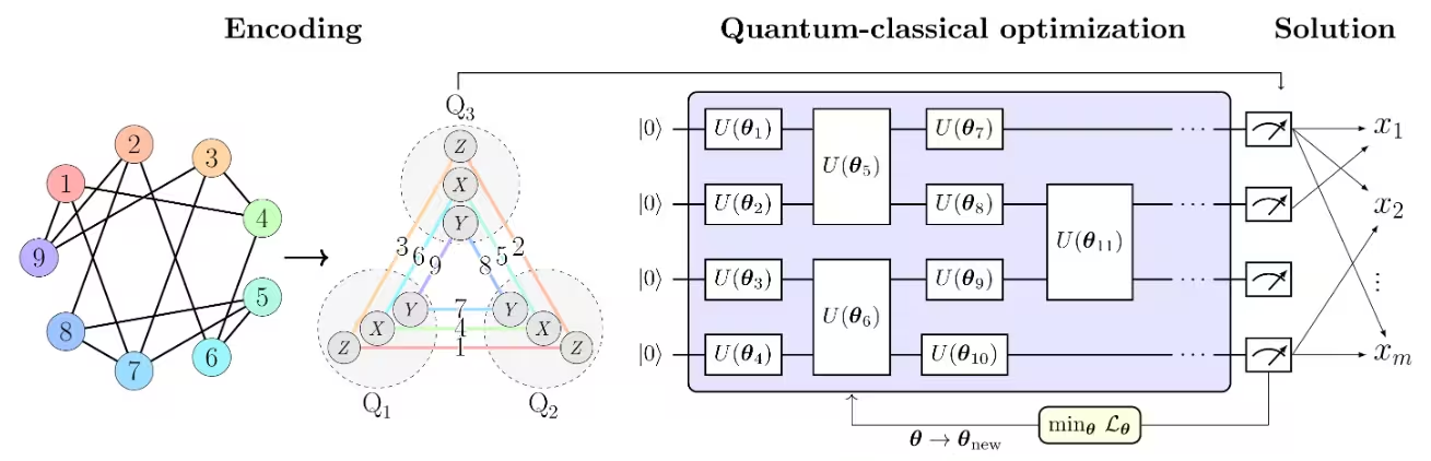
I dr Abbildig 1 us [1] wird s'Max-Cut-Problem als Bispiil bruucht, zum de PCE-Aasatz z'illustriere. S'Max-Cut-Problem mit $m=9$ Chnoote wird in ene Pauli-Korrelationsraum kodiert und stellt s'Optimierigsproblem als Korrelationsmatrix dar — konkret: 2-Körper-Pauli-Matrix-Korrelationen über $n=3$ Qubits $(Q_1, Q_2, Q_3)$. D'Farbig vo de Chnoote zeigt de Pauli-String, wo für jede kodierte Chnote bruucht wird.

Zum Bispiil wird Chnote 1, wo dr binäre Variable $x_1$ entspricht, dur de Erwärtigswärt vo $Z_1 \otimes Z_2 \otimes I_3$ kodiert, während $x_8$ dur $I_1 \otimes Y_2 \otimes Y_3$ verschlüsslet wird. Das entspricht emere Kompressio vo de $m$ Variable vom Problem i $n = O(m^{1/2})$ Qubits. Allgemein ermögliche $k$-Körper-Korrelationen polynomiale Kompressione vo dr Ordnig $k$. Dr gwählti Pauli-Satz bstäit us drüü Teilmengen vo gegesitig kommutierendi Pauli-Strings, was s'Schätze vo allne $m$ Korrelationen mit numme drüü Mässigsiistellige ermöglicht.

E Verlustfunktion $\mathcal{L}$ us Pauli-Erwärtigswärt, wo d'ursprünglich Max-Cut-Zielfunktion nachahmt, wird konstruiert. D'Verlustfunktion wird denn mit emene quanteklassische Optimierigslöser wie em Variational Quantum Eigensolver (VQE) optimiert.

Sobald d'Optimierig abgschlosse isch, wird d'Lösig zrugg in de ursprüngliche Optimierigsproblemraum dekodiert, was d'optimali Max-Cut-Lösig liifert.

Vorussetzige

Bevor du mit däm Tutorial aafangsch, stell sicher, dass du s'Folgendi iigschtallt häsch:

• Qiskit SDK v1.0 oder neuer, mit Unterstützig für Visualisierig
• Qiskit Runtime v0.22 oder neuer (pip install qiskit-ibm-runtime)

Setup

# Added by doQumentation — installs packages not in the Binder environment
!pip install -q networkx

from itertools import combinations

import numpy as np
import rustworkx as rx
from scipy.optimize import minimize

from qiskit.circuit.library import efficient_su2
from qiskit.transpiler.preset_passmanagers import generate_preset_pass_manager
from qiskit.quantum_info import SparsePauliOp
from qiskit_ibm_runtime import EstimatorV2 as Estimator
from qiskit_ibm_runtime import QiskitRuntimeService
from qiskit_ibm_runtime import Session
from rustworkx.visualization import mpl_draw

service = QiskitRuntimeService()
backend = service.least_busy(
    operational=True, simulator=False, min_num_qubits=127
)

def calc_cut_size(graph, partition0, partition1):
    """Calculate the cut size of the given partitions of the graph."""

    cut_size = 0
    for edge0, edge1 in graph.edge_list():
        if edge0 in partition0 and edge1 in partition1:
            cut_size += 1
        elif edge0 in partition1 and edge1 in partition0:
            cut_size += 1
    return cut_size

Schritt 1: Klassischi Iigab uf es Quanteproblem abbilden

Max-Cut-Problem

S'Max-Cut-Problem isch es kombinatorisches Optimierigsproblem, wo uf emene Graph $G = (V, E)$ definiert isch, wo $V$ d'Menge vo de Eckpunkte und $E$ d'Menge vo de Chante isch. S'Ziel isch, d'Eckpunkte in zwee Menge, $S$ und $V \setminus S$, z'underteile, so dass d'Aazahl vo de Chante zwüsche de zwei Menge maximiert wird. Für e detaillierti Bschribig vom Max-Cut-Problem, lueg bitte im Tutorial "Quantum Approximate Optimization Algorithm" nooch. S'Max-Cut-Problem wird au als Bispiil im Tutorial "Fortgschritteni Technike für QAOA" bruucht. I jene Tutorials wird dr QAOA-Algorithmus bruucht, zum s'Max-Cut-Problem z'löse.

Graph -> Hamiltonian

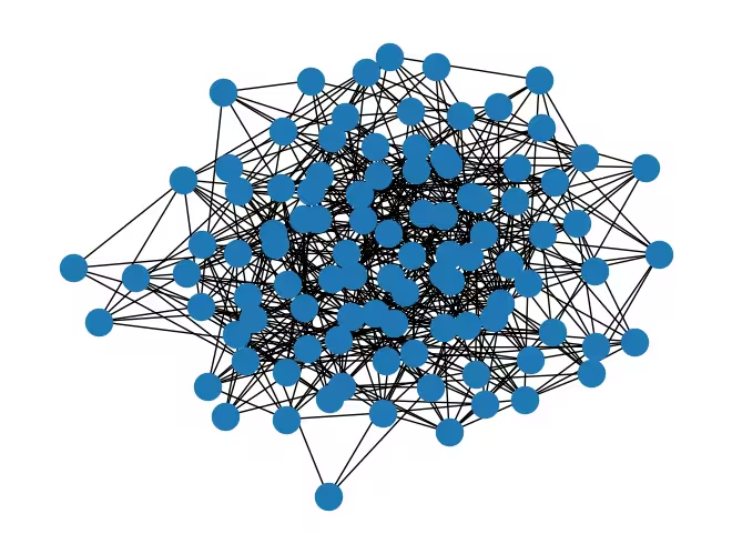
Dises Tutorial bruucht ene zufälligi Graph mit 1000 Chnoote.

D'Problemgrösse isch schwer z'visualisiere, drum isch unten e Graph mit 100 Chnoote z'gsee. (E Graph mit 1000 Chnoote direkt z'rändere wär z'diicht, um irgendöppis z'erkenne!) Dr Graph, mit däm mir arbyte, isch zehnmal so gross.

mpl_draw(rx.undirected_gnp_random_graph(100, 0.1, seed=42))

num_nodes = 1000  # Number of nodes in graph
graph = rx.undirected_gnp_random_graph(num_nodes, 0.1, seed=42)

import networkx as nx

nx_graph = nx.Graph()
nx_graph.add_nodes_from(range(num_nodes))

for edge in graph.edge_list():
    nx_graph.add_edge(edge[0], edge[1])

curr_cut_size, partition = nx.approximation.one_exchange(nx_graph, seed=1)
print(f"Initial cut size: {curr_cut_size}")

Initial cut size: 28075

Mir kodiere de Graph mit 1000 Chnoote i 2-Körper-Pauli-Matrix-Korrelationen über 100 Qubits. Dr Graph wird als Korrelationsmatrix dargschtellt, wo jede Chnote dur ene Pauli-String kodiert wird. S'Vorzeiche vom Erwärtigswärt vom Pauli-String zeigt d'Zueghörigkeit vo dr Chnote zu enere Partition. Zum Bispiil wird Chnote 0 dur ene Pauli-String $\prod_0 = I_{19} \otimes ... I_2 \otimes X_1 \otimes X_0$ kodiert. S'Vorzeiche vom Erwärtigswärt vo däm Pauli-String zeigt d'Partition vo Chnote 0 aa. Mir definiere e Pauli-Korrelationscodierig (PCE) relativ zu $\prod$ als

$x_i \coloneqq \textit{sgn}(\langle\prod_i \rangle)$

wo $x_i$ d'Partition vo Chnote $i$ isch und $\langle \prod_i \rangle \coloneqq \langle \psi |\prod_i| \psi \rangle$ dr Erwärtigswärt vom Pauli-String isch, wo Chnote $i$ über ene Quantezuestand $|\psi \rangle$ kodiert. Jetzt codiere mir de Graph i ene Hamiltonian mit PCE. Mir unterteile d'Chnoote in drüü Menge: $S_1$, $S_2$ und $S_3$. Dann verschlüssle mir d'Chnoote in jedere Menge mit de Pauli-Strings $X$, $Y$ bzw. $Z$.

num_qubits = 100

list_size = num_nodes // 3
node_x = [i for i in range(list_size)]
node_y = [i for i in range(list_size, 2 * list_size)]
node_z = [i for i in range(2 * list_size, num_nodes)]

print("List 1:", node_x)
print("List 2:", node_y)
print("List 3:", node_z)

List 1: [0, 1, 2, 3, 4, 5, 6, 7, 8, 9, 10, 11, 12, 13, 14, 15, 16, 17, 18, 19, 20, 21, 22, 23, 24, 25, 26, 27, 28, 29, 30, 31, 32, 33, 34, 35, 36, 37, 38, 39, 40, 41, 42, 43, 44, 45, 46, 47, 48, 49, 50, 51, 52, 53, 54, 55, 56, 57, 58, 59, 60, 61, 62, 63, 64, 65, 66, 67, 68, 69, 70, 71, 72, 73, 74, 75, 76, 77, 78, 79, 80, 81, 82, 83, 84, 85, 86, 87, 88, 89, 90, 91, 92, 93, 94, 95, 96, 97, 98, 99, 100, 101, 102, 103, 104, 105, 106, 107, 108, 109, 110, 111, 112, 113, 114, 115, 116, 117, 118, 119, 120, 121, 122, 123, 124, 125, 126, 127, 128, 129, 130, 131, 132, 133, 134, 135, 136, 137, 138, 139, 140, 141, 142, 143, 144, 145, 146, 147, 148, 149, 150, 151, 152, 153, 154, 155, 156, 157, 158, 159, 160, 161, 162, 163, 164, 165, 166, 167, 168, 169, 170, 171, 172, 173, 174, 175, 176, 177, 178, 179, 180, 181, 182, 183, 184, 185, 186, 187, 188, 189, 190, 191, 192, 193, 194, 195, 196, 197, 198, 199, 200, 201, 202, 203, 204, 205, 206, 207, 208, 209, 210, 211, 212, 213, 214, 215, 216, 217, 218, 219, 220, 221, 222, 223, 224, 225, 226, 227, 228, 229, 230, 231, 232, 233, 234, 235, 236, 237, 238, 239, 240, 241, 242, 243, 244, 245, 246, 247, 248, 249, 250, 251, 252, 253, 254, 255, 256, 257, 258, 259, 260, 261, 262, 263, 264, 265, 266, 267, 268, 269, 270, 271, 272, 273, 274, 275, 276, 277, 278, 279, 280, 281, 282, 283, 284, 285, 286, 287, 288, 289, 290, 291, 292, 293, 294, 295, 296, 297, 298, 299, 300, 301, 302, 303, 304, 305, 306, 307, 308, 309, 310, 311, 312, 313, 314, 315, 316, 317, 318, 319, 320, 321, 322, 323, 324, 325, 326, 327, 328, 329, 330, 331, 332]
List 2: [333, 334, 335, 336, 337, 338, 339, 340, 341, 342, 343, 344, 345, 346, 347, 348, 349, 350, 351, 352, 353, 354, 355, 356, 357, 358, 359, 360, 361, 362, 363, 364, 365, 366, 367, 368, 369, 370, 371, 372, 373, 374, 375, 376, 377, 378, 379, 380, 381, 382, 383, 384, 385, 386, 387, 388, 389, 390, 391, 392, 393, 394, 395, 396, 397, 398, 399, 400, 401, 402, 403, 404, 405, 406, 407, 408, 409, 410, 411, 412, 413, 414, 415, 416, 417, 418, 419, 420, 421, 422, 423, 424, 425, 426, 427, 428, 429, 430, 431, 432, 433, 434, 435, 436, 437, 438, 439, 440, 441, 442, 443, 444, 445, 446, 447, 448, 449, 450, 451, 452, 453, 454, 455, 456, 457, 458, 459, 460, 461, 462, 463, 464, 465, 466, 467, 468, 469, 470, 471, 472, 473, 474, 475, 476, 477, 478, 479, 480, 481, 482, 483, 484, 485, 486, 487, 488, 489, 490, 491, 492, 493, 494, 495, 496, 497, 498, 499, 500, 501, 502, 503, 504, 505, 506, 507, 508, 509, 510, 511, 512, 513, 514, 515, 516, 517, 518, 519, 520, 521, 522, 523, 524, 525, 526, 527, 528, 529, 530, 531, 532, 533, 534, 535, 536, 537, 538, 539, 540, 541, 542, 543, 544, 545, 546, 547, 548, 549, 550, 551, 552, 553, 554, 555, 556, 557, 558, 559, 560, 561, 562, 563, 564, 565, 566, 567, 568, 569, 570, 571, 572, 573, 574, 575, 576, 577, 578, 579, 580, 581, 582, 583, 584, 585, 586, 587, 588, 589, 590, 591, 592, 593, 594, 595, 596, 597, 598, 599, 600, 601, 602, 603, 604, 605, 606, 607, 608, 609, 610, 611, 612, 613, 614, 615, 616, 617, 618, 619, 620, 621, 622, 623, 624, 625, 626, 627, 628, 629, 630, 631, 632, 633, 634, 635, 636, 637, 638, 639, 640, 641, 642, 643, 644, 645, 646, 647, 648, 649, 650, 651, 652, 653, 654, 655, 656, 657, 658, 659, 660, 661, 662, 663, 664, 665]
List 3: [666, 667, 668, 669, 670, 671, 672, 673, 674, 675, 676, 677, 678, 679, 680, 681, 682, 683, 684, 685, 686, 687, 688, 689, 690, 691, 692, 693, 694, 695, 696, 697, 698, 699, 700, 701, 702, 703, 704, 705, 706, 707, 708, 709, 710, 711, 712, 713, 714, 715, 716, 717, 718, 719, 720, 721, 722, 723, 724, 725, 726, 727, 728, 729, 730, 731, 732, 733, 734, 735, 736, 737, 738, 739, 740, 741, 742, 743, 744, 745, 746, 747, 748, 749, 750, 751, 752, 753, 754, 755, 756, 757, 758, 759, 760, 761, 762, 763, 764, 765, 766, 767, 768, 769, 770, 771, 772, 773, 774, 775, 776, 777, 778, 779, 780, 781, 782, 783, 784, 785, 786, 787, 788, 789, 790, 791, 792, 793, 794, 795, 796, 797, 798, 799, 800, 801, 802, 803, 804, 805, 806, 807, 808, 809, 810, 811, 812, 813, 814, 815, 816, 817, 818, 819, 820, 821, 822, 823, 824, 825, 826, 827, 828, 829, 830, 831, 832, 833, 834, 835, 836, 837, 838, 839, 840, 841, 842, 843, 844, 845, 846, 847, 848, 849, 850, 851, 852, 853, 854, 855, 856, 857, 858, 859, 860, 861, 862, 863, 864, 865, 866, 867, 868, 869, 870, 871, 872, 873, 874, 875, 876, 877, 878, 879, 880, 881, 882, 883, 884, 885, 886, 887, 888, 889, 890, 891, 892, 893, 894, 895, 896, 897, 898, 899, 900, 901, 902, 903, 904, 905, 906, 907, 908, 909, 910, 911, 912, 913, 914, 915, 916, 917, 918, 919, 920, 921, 922, 923, 924, 925, 926, 927, 928, 929, 930, 931, 932, 933, 934, 935, 936, 937, 938, 939, 940, 941, 942, 943, 944, 945, 946, 947, 948, 949, 950, 951, 952, 953, 954, 955, 956, 957, 958, 959, 960, 961, 962, 963, 964, 965, 966, 967, 968, 969, 970, 971, 972, 973, 974, 975, 976, 977, 978, 979, 980, 981, 982, 983, 984, 985, 986, 987, 988, 989, 990, 991, 992, 993, 994, 995, 996, 997, 998, 999]

def build_pauli_correlation_encoding(pauli, node_list, n, k=2):
    pauli_correlation_encoding = []
    for idx, c in enumerate(combinations(range(n), k)):
        if idx >= len(node_list):
            break
        paulis = ["I"] * n
        paulis[c[0]], paulis[c[1]] = pauli, pauli
        pauli_correlation_encoding.append(("".join(paulis)[::-1], 1))

    hamiltonian = []
    for pauli, weight in pauli_correlation_encoding:
        hamiltonian.append(SparsePauliOp.from_list([(pauli, weight)]))

    return hamiltonian

pauli_correlation_encoding_x = build_pauli_correlation_encoding(
    "X", node_x, num_qubits
)
pauli_correlation_encoding_y = build_pauli_correlation_encoding(
    "Y", node_y, num_qubits
)
pauli_correlation_encoding_z = build_pauli_correlation_encoding(
    "Z", node_z, num_qubits
)

Schritt 2: Problem für d'Quantehardware-Uusfüehrig optimiere

Quantum Circuit

Do wird de Zuestand $|\psi \rangle$ mit $\mathbf{\theta}$ parametrisiert, und mir optimiere die Parameter $\mathbf{\theta}$ mit emene variationelle Aasatz. Dises Tutorial setzt de efficient_su2-Ansatz für de variationelle Algorithmus ii, wäge sinere Uusdrucksstärchi und Iifachheit bi dr Implementierig. Mir bruuche au d'relaxierti Verlustfunktion, wo spöter in däm Tutorial vorgschtellt wird. Dadur chöne mir grossmassstäbigi Probleem mit weniger Qubits und flachere Schaltkreistiifene lösä.

# Build the quantum circuit
qc = efficient_su2(num_qubits, ["ry", "rz"], reps=2)

# Optimize the circuit

pm = generate_preset_pass_manager(optimization_level=3, backend=backend)
qc = pm.run(qc)

Verlustfunktion

Für d'Verlustfunktion $\mathcal{L}$ bruuche mir e Relaxierig vo dr Max-Cut-Zielfunktion, wie i [1] bschriibe, wo als $\mathcal{V}(\mathbf{x}) \coloneqq \sum_{(i, j) \in E} W_{i, j}(1-x_i x_j)$ definiert isch. Do bezeichnet $W_{i, j}$ s'Gwicht vo dr Chante $(i, j)$, und $x_i$ stellt d'Partition vo Chnote $i$ dar. D'Verlustfunktion $\mathcal{L}$ isch definiert als:

$\mathcal{L}\coloneqq \sum_{(i, j) \in E} W_{i, j} \text{tanh} (\alpha \langle\prod_i \rangle) \text{tanh} (\alpha \langle\prod_j \rangle) + \mathcal{L}^{(\text{reg})}$

wo d'Max-Cut-Zielfunktion dur d'glatte hyperbolische Tangens vo de Erwärtigswärt vo de Pauli-Strings, wo d'Chnoote kodiere, ersetzt wird. Dr Regularisierigstärm $\mathcal{L}^{(\text{reg})}$ und dr Skalifaktor $\alpha$, proportional zur Aazahl vo Qubits, wärde iigeführt, zum d'Leistig vom Löser z'verbessere.

Dr Regularisierigstärm isch definiert als:

$\mathcal{L}^{(\text{reg})}$ isch definiert als $\mathcal{L}^{(\text{reg})} \coloneqq \beta \nu \lbrack \frac{1}{m} \sum_{i \in V} \text{tanh} (\alpha \langle\prod_i \rangle)^2 \rbrack ^2$

wo $\beta=1/2$, $\nu = |E|/2 + (m -1) /4$, und $m$ d'Aazahl vo de Chnoote im Graph isch.

def loss_func_estimator(x, ansatz, hamiltonian, estimator, graph):
    """
    Calculates the specified loss function for the given ansatz, Hamiltonian, and graph.

    The expectation values of each Pauli string in the Hamiltonian are first obtained
    by running the ansatz on the quantum backend. These expectation values are then
    passed through the nonlinear function tanh(alpha * prod_i). The loss function is
    subsequently computed from these transformed values.
    """
    job = estimator.run(
        [
            (ansatz, hamiltonian[0], x),
            (ansatz, hamiltonian[1], x),
            (ansatz, hamiltonian[2], x),
        ]
    )
    result = job.result()

    # calculate the loss function
    node_exp_map = {}
    idx = 0
    for r in result:
        for ev in r.data.evs:
            node_exp_map[idx] = ev
            idx += 1

    loss = 0
    alpha = num_qubits
    for edge0, edge1 in graph.edge_list():
        loss += np.tanh(alpha * node_exp_map[edge0]) * np.tanh(
            alpha * node_exp_map[edge1]
        )

    regulation_term = 0
    for i in range(len(graph.nodes())):
        regulation_term += np.tanh(alpha * node_exp_map[i]) ** 2
    regulation_term = regulation_term / len(graph.nodes())
    regulation_term = regulation_term**2
    beta = 1 / 2
    v = len(graph.edges()) / 2 + (len(graph.nodes()) - 1) / 4
    regulation_term = beta * v * regulation_term

    loss = loss + regulation_term

    global experiment_result
    print(f"Iter {len(experiment_result)}: {loss}")
    experiment_result.append({"loss": loss, "exp_map": node_exp_map})
    return loss

Schritt 3: Mit Qiskit-Primitive uusfüehre

I däm Tutorial setze mir max_iter=50 für de Optimierigsdurchgang als Demonstrationszwäck. Wenn mir d'Aazahl vo de Iteratione erhöhe, chöne mir bässe Ergebnis erwartte.

pce = []
pce.append(
    [op.apply_layout(qc.layout) for op in pauli_correlation_encoding_x]
)
pce.append(
    [op.apply_layout(qc.layout) for op in pauli_correlation_encoding_y]
)
pce.append(
    [op.apply_layout(qc.layout) for op in pauli_correlation_encoding_z]
)

# Run the optimization using Session

with Session(backend=backend) as session:
    estimator = Estimator(mode=session)

    experiment_result = []

    def loss_func(x):
        return loss_func_estimator(
            x, qc, [pce[0], pce[1], pce[2]], estimator, graph
        )

    np.random.seed(42)
    initial_params = np.random.rand(qc.num_parameters)
    result = minimize(
        loss_func, initial_params, method="COBYLA", options={"maxiter": 50}
    )
print(result)

Iter 0: 16659.649201600296
Iter 1: 12104.242957555361
Iter 2: 6541.137221994661
Iter 3: 6650.6188244671985
Iter 4: 7033.193518185085
Iter 5: 6743.687931793412
Iter 6: 6223.574718684094
Iter 7: 6457.3302709535965
Iter 8: 6581.316449107595
Iter 9: 6365.761052029896
Iter 10: 6415.872673527322
Iter 11: 6421.996561600348
Iter 12: 6636.372822791712
Iter 13: 6965.174320702346
Iter 14: 6774.236562696287
Iter 15: 6393.837617108355
Iter 16: 6234.311401676519
Iter 17: 6518.192237615901
Iter 18: 6559.933925068997
Iter 19: 6646.157979243488
Iter 20: 6573.726111605048
Iter 21: 6190.642092901959
Iter 22: 6653.06500163594
Iter 23: 6545.713700369988
Iter 24: 6399.996441760465
Iter 25: 6115.959687941808
Iter 26: 6665.915093554849
Iter 27: 6832.882201259893
Iter 28: 6541.392749578919
Iter 29: 6813.3456910443165
Iter 30: 6460.800944368402
Iter 31: 6359.635437029245
Iter 32: 6040.891641882451
Iter 33: 6573.930674936448
Iter 34: 6668.031753293785
Iter 35: 6450.002712889748
Iter 36: 6519.8298811058075
Iter 37: 6467.134502398199
Iter 38: 6655.284651397334
Iter 39: 6371.168353987336
Iter 40: 6480.337259347923
Iter 41: 6339.256786764425
Iter 42: 6588.635046825541
Iter 43: 6617.677964971322
Iter 44: 6469.0441600679205
Iter 45: 6567.874244906106
Iter 46: 6217.899975264532
Iter 47: 6783.481394627947
Iter 48: 6813.371853626112
Iter 49: 6506.5871531488765
 message: Maximum number of function evaluations has been exceeded.
 success: False
  status: 2
     fun: 6040.891641882451
       x: [ 1.375e+00  1.951e+00 ...  1.923e-01  4.087e-02]
    nfev: 50
   maxcv: 0.0

Schritt 4: Ergebnis noochbearbeite und im gwünschte klassische Format zruggge

D'Partitione vo de Chnoote wärde bestimmt, indem s'Vorzeiche vo de Erwärtigswärt vo de Pauli-Strings, wo d'Chnoote codiere, uusgwertet wird.

# Calculate the partitions based on the final expectation values
# If the expectation value is positive, the node belongs to partition 0 (par0)
# Otherwise, the node belongs to partition 1 (par1)

par0, par1 = set(), set()

for i in experiment_result[-1]["exp_map"]:
    if experiment_result[-1]["exp_map"][i] >= 0:
        par0.add(i)
    else:
        par1.add(i)
print(par0, par1)

{0, 1, 4, 8, 9, 10, 12, 13, 14, 15, 16, 18, 25, 27, 31, 32, 34, 36, 38, 39, 40, 41, 44, 46, 47, 48, 49, 50, 51, 52, 57, 60, 61, 62, 63, 64, 65, 66, 68, 71, 79, 81, 82, 86, 88, 91, 92, 93, 94, 95, 96, 99, 100, 105, 106, 107, 112, 114, 115, 121, 123, 129, 133, 134, 145, 147, 161, 165, 166, 168, 171, 173, 184, 185, 187, 188, 192, 193, 194, 196, 197, 198, 202, 205, 206, 207, 208, 209, 210, 211, 215, 217, 218, 219, 220, 221, 225, 226, 227, 228, 229, 230, 231, 232, 233, 234, 235, 236, 238, 241, 242, 243, 244, 246, 247, 248, 249, 251, 252, 253, 255, 256, 257, 258, 259, 261, 262, 264, 265, 266, 268, 269, 270, 272, 273, 275, 276, 277, 278, 279, 281, 283, 284, 285, 286, 288, 292, 293, 294, 299, 300, 303, 305, 306, 307, 308, 310, 312, 313, 314, 316, 317, 319, 321, 326, 327, 328, 333, 336, 338, 340, 341, 342, 344, 345, 346, 349, 351, 352, 353, 356, 357, 360, 361, 362, 363, 364, 366, 368, 370, 374, 378, 379, 380, 381, 382, 383, 384, 386, 387, 388, 389, 390, 391, 393, 394, 395, 396, 397, 398, 404, 405, 406, 409, 411, 413, 415, 416, 418, 421, 425, 426, 427, 428, 429, 433, 434, 435, 437, 444, 450, 456, 457, 458, 459, 462, 463, 465, 467, 469, 470, 472, 476, 479, 484, 487, 489, 492, 493, 497, 498, 499, 502, 506, 508, 513, 516, 517, 518, 519, 521, 523, 526, 527, 528, 531, 532, 533, 535, 536, 537, 539, 540, 541, 542, 543, 544, 545, 547, 549, 550, 552, 557, 562, 563, 564, 565, 567, 568, 569, 570, 571, 572, 573, 576, 578, 579, 580, 583, 585, 587, 588, 589, 591, 595, 596, 597, 600, 602, 603, 604, 605, 606, 607, 608, 609, 610, 612, 618, 619, 623, 624, 625, 626, 627, 628, 630, 632, 636, 637, 640, 644, 646, 649, 652, 656, 657, 658, 659, 661, 662, 663, 664, 667, 669, 670, 671, 672, 674, 675, 676, 677, 678, 679, 680, 681, 682, 683, 684, 685, 686, 687, 688, 689, 690, 692, 693, 694, 695, 696, 698, 700, 701, 703, 706, 707, 708, 709, 712, 713, 714, 716, 717, 718, 719, 721, 722, 723, 724, 725, 726, 728, 730, 731, 733, 734, 735, 737, 739, 740, 741, 743, 744, 746, 748, 750, 751, 752, 753, 754, 758, 760, 761, 762, 763, 764, 765, 766, 774, 778, 780, 782, 787, 795, 800, 802, 803, 808, 809, 812, 818, 822, 825, 827, 834, 836, 840, 843, 845, 847, 850, 853, 854, 857, 858, 863, 864, 865, 866, 867, 868, 869, 870, 872, 873, 874, 875, 876, 878, 880, 881, 882, 883, 884, 885, 887, 888, 889, 890, 891, 893, 894, 895, 896, 898, 901, 902, 903, 904, 905, 907, 908, 910, 911, 912, 913, 914, 915, 916, 917, 918, 920, 921, 923, 925, 926, 928, 929, 930, 932, 934, 935, 936, 938, 939, 941, 943, 945, 946, 947, 948, 949, 953, 955, 956, 957, 958, 959, 961, 966, 975, 978, 980, 983, 988, 990, 996, 999} {2, 3, 5, 6, 7, 11, 17, 19, 20, 21, 22, 23, 24, 26, 28, 29, 30, 33, 35, 37, 42, 43, 45, 53, 54, 55, 56, 58, 59, 67, 69, 70, 72, 73, 74, 75, 76, 77, 78, 80, 83, 84, 85, 87, 89, 90, 97, 98, 101, 102, 103, 104, 108, 109, 110, 111, 113, 116, 117, 118, 119, 120, 122, 124, 125, 126, 127, 128, 130, 131, 132, 135, 136, 137, 138, 139, 140, 141, 142, 143, 144, 146, 148, 149, 150, 151, 152, 153, 154, 155, 156, 157, 158, 159, 160, 162, 163, 164, 167, 169, 170, 172, 174, 175, 176, 177, 178, 179, 180, 181, 182, 183, 186, 189, 190, 191, 195, 199, 200, 201, 203, 204, 212, 213, 214, 216, 222, 223, 224, 237, 239, 240, 245, 250, 254, 260, 263, 267, 271, 274, 280, 282, 287, 289, 290, 291, 295, 296, 297, 298, 301, 302, 304, 309, 311, 315, 318, 320, 322, 323, 324, 325, 329, 330, 331, 332, 334, 335, 337, 339, 343, 347, 348, 350, 354, 355, 358, 359, 365, 367, 369, 371, 372, 373, 375, 376, 377, 385, 392, 399, 400, 401, 402, 403, 407, 408, 410, 412, 414, 417, 419, 420, 422, 423, 424, 430, 431, 432, 436, 438, 439, 440, 441, 442, 443, 445, 446, 447, 448, 449, 451, 452, 453, 454, 455, 460, 461, 464, 466, 468, 471, 473, 474, 475, 477, 478, 480, 481, 482, 483, 485, 486, 488, 490, 491, 494, 495, 496, 500, 501, 503, 504, 505, 507, 509, 510, 511, 512, 514, 515, 520, 522, 524, 525, 529, 530, 534, 538, 546, 548, 551, 553, 554, 555, 556, 558, 559, 560, 561, 566, 574, 575, 577, 581, 582, 584, 586, 590, 592, 593, 594, 598, 599, 601, 611, 613, 614, 615, 616, 617, 620, 621, 622, 629, 631, 633, 634, 635, 638, 639, 641, 642, 643, 645, 647, 648, 650, 651, 653, 654, 655, 660, 665, 666, 668, 673, 691, 697, 699, 702, 704, 705, 710, 711, 715, 720, 727, 729, 732, 736, 738, 742, 745, 747, 749, 755, 756, 757, 759, 767, 768, 769, 770, 771, 772, 773, 775, 776, 777, 779, 781, 783, 784, 785, 786, 788, 789, 790, 791, 792, 793, 794, 796, 797, 798, 799, 801, 804, 805, 806, 807, 810, 811, 813, 814, 815, 816, 817, 819, 820, 821, 823, 824, 826, 828, 829, 830, 831, 832, 833, 835, 837, 838, 839, 841, 842, 844, 846, 848, 849, 851, 852, 855, 856, 859, 860, 861, 862, 871, 877, 879, 886, 892, 897, 899, 900, 906, 909, 919, 922, 924, 927, 931, 933, 937, 940, 942, 944, 950, 951, 952, 954, 960, 962, 963, 964, 965, 967, 968, 969, 970, 971, 972, 973, 974, 976, 977, 979, 981, 982, 984, 985, 986, 987, 989, 991, 992, 993, 994, 995, 997, 998}

Mir chöne d'Schnittgrösse vom Max-Cut-Problem mit de Partitione vo de Chnoote berechne.

cut_size = calc_cut_size(graph, par0, par1)
print(f"Cut size: {cut_size}")

Cut size: 24682

Sobald s'Training abgschlossen isch, füehre mir e Runde Einzelbit-Swap-Suechi us, zum d'Lösig als klassische Noochbearbeitigsschritt z'verbessere. I däm Prozess tausche mir d'Partitione vo zwei Chnoote und berechne d'Schnittgrösse. Wenn d'Schnittgrösse besser wird, bhalte mir de Tausch. Mir widerhole de Prozess für alli mögliche Paare vo Chnoote, wo dur e Chante verbunde sind.

best_bits = []
cur_bits = []

for i in experiment_result[-1]["exp_map"]:
    if experiment_result[-1]["exp_map"][i] >= 0:
        cur_bits.append(1)
    else:
        cur_bits.append(0)
print(cur_bits)

[1, 1, 0, 0, 1, 0, 0, 0, 1, 1, 1, 0, 1, 1, 1, 1, 1, 0, 1, 0, 0, 0, 0, 0, 0, 1, 0, 1, 0, 0, 0, 1, 1, 0, 1, 0, 1, 0, 1, 1, 1, 1, 0, 0, 1, 0, 1, 1, 1, 1, 1, 1, 1, 0, 0, 0, 0, 1, 0, 0, 1, 1, 1, 1, 1, 1, 1, 0, 1, 0, 0, 1, 0, 0, 0, 0, 0, 0, 0, 1, 0, 1, 1, 0, 0, 0, 1, 0, 1, 0, 0, 1, 1, 1, 1, 1, 1, 0, 0, 1, 1, 0, 0, 0, 0, 1, 1, 1, 0, 0, 0, 0, 1, 0, 1, 1, 0, 0, 0, 0, 0, 1, 0, 1, 0, 0, 0, 0, 0, 1, 0, 0, 0, 1, 1, 0, 0, 0, 0, 0, 0, 0, 0, 0, 0, 1, 0, 1, 0, 0, 0, 0, 0, 0, 0, 0, 0, 0, 0, 0, 0, 1, 0, 0, 0, 1, 1, 0, 1, 0, 0, 1, 0, 1, 0, 0, 0, 0, 0, 0, 0, 0, 0, 0, 1, 1, 0, 1, 1, 0, 0, 0, 1, 1, 1, 0, 1, 1, 1, 0, 0, 0, 1, 0, 0, 1, 1, 1, 1, 1, 1, 1, 0, 0, 0, 1, 0, 1, 1, 1, 1, 1, 0, 0, 0, 1, 1, 1, 1, 1, 1, 1, 1, 1, 1, 1, 1, 0, 1, 0, 0, 1, 1, 1, 1, 0, 1, 1, 1, 1, 0, 1, 1, 1, 0, 1, 1, 1, 1, 1, 0, 1, 1, 0, 1, 1, 1, 0, 1, 1, 1, 0, 1, 1, 0, 1, 1, 1, 1, 1, 0, 1, 0, 1, 1, 1, 1, 0, 1, 0, 0, 0, 1, 1, 1, 0, 0, 0, 0, 1, 1, 0, 0, 1, 0, 1, 1, 1, 1, 0, 1, 0, 1, 1, 1, 0, 1, 1, 0, 1, 0, 1, 0, 0, 0, 0, 1, 1, 1, 0, 0, 0, 0, 1, 0, 0, 1, 0, 1, 0, 1, 1, 1, 0, 1, 1, 1, 0, 0, 1, 0, 1, 1, 1, 0, 0, 1, 1, 0, 0, 1, 1, 1, 1, 1, 0, 1, 0, 1, 0, 1, 0, 0, 0, 1, 0, 0, 0, 1, 1, 1, 1, 1, 1, 1, 0, 1, 1, 1, 1, 1, 1, 0, 1, 1, 1, 1, 1, 1, 0, 0, 0, 0, 0, 1, 1, 1, 0, 0, 1, 0, 1, 0, 1, 0, 1, 1, 0, 1, 0, 0, 1, 0, 0, 0, 1, 1, 1, 1, 1, 0, 0, 0, 1, 1, 1, 0, 1, 0, 0, 0, 0, 0, 0, 1, 0, 0, 0, 0, 0, 1, 0, 0, 0, 0, 0, 1, 1, 1, 1, 0, 0, 1, 1, 0, 1, 0, 1, 0, 1, 1, 0, 1, 0, 0, 0, 1, 0, 0, 1, 0, 0, 0, 0, 1, 0, 0, 1, 0, 1, 0, 0, 1, 1, 0, 0, 0, 1, 1, 1, 0, 0, 1, 0, 0, 0, 1, 0, 1, 0, 0, 0, 0, 1, 0, 0, 1, 1, 1, 1, 0, 1, 0, 1, 0, 0, 1, 1, 1, 0, 0, 1, 1, 1, 0, 1, 1, 1, 0, 1, 1, 1, 1, 1, 1, 1, 0, 1, 0, 1, 1, 0, 1, 0, 0, 0, 0, 1, 0, 0, 0, 0, 1, 1, 1, 1, 0, 1, 1, 1, 1, 1, 1, 1, 0, 0, 1, 0, 1, 1, 1, 0, 0, 1, 0, 1, 0, 1, 1, 1, 0, 1, 0, 0, 0, 1, 1, 1, 0, 0, 1, 0, 1, 1, 1, 1, 1, 1, 1, 1, 1, 0, 1, 0, 0, 0, 0, 0, 1, 1, 0, 0, 0, 1, 1, 1, 1, 1, 1, 0, 1, 0, 1, 0, 0, 0, 1, 1, 0, 0, 1, 0, 0, 0, 1, 0, 1, 0, 0, 1, 0, 0, 1, 0, 0, 0, 1, 1, 1, 1, 0, 1, 1, 1, 1, 0, 0, 1, 0, 1, 1, 1, 1, 0, 1, 1, 1, 1, 1, 1, 1, 1, 1, 1, 1, 1, 1, 1, 1, 1, 1, 0, 1, 1, 1, 1, 1, 0, 1, 0, 1, 1, 0, 1, 0, 0, 1, 1, 1, 1, 0, 0, 1, 1, 1, 0, 1, 1, 1, 1, 0, 1, 1, 1, 1, 1, 1, 0, 1, 0, 1, 1, 0, 1, 1, 1, 0, 1, 0, 1, 1, 1, 0, 1, 1, 0, 1, 0, 1, 0, 1, 1, 1, 1, 1, 0, 0, 0, 1, 0, 1, 1, 1, 1, 1, 1, 1, 0, 0, 0, 0, 0, 0, 0, 1, 0, 0, 0, 1, 0, 1, 0, 1, 0, 0, 0, 0, 1, 0, 0, 0, 0, 0, 0, 0, 1, 0, 0, 0, 0, 1, 0, 1, 1, 0, 0, 0, 0, 1, 1, 0, 0, 1, 0, 0, 0, 0, 0, 1, 0, 0, 0, 1, 0, 0, 1, 0, 1, 0, 0, 0, 0, 0, 0, 1, 0, 1, 0, 0, 0, 1, 0, 0, 1, 0, 1, 0, 1, 0, 0, 1, 0, 0, 1, 1, 0, 0, 1, 1, 0, 0, 0, 0, 1, 1, 1, 1, 1, 1, 1, 1, 0, 1, 1, 1, 1, 1, 0, 1, 0, 1, 1, 1, 1, 1, 1, 0, 1, 1, 1, 1, 1, 0, 1, 1, 1, 1, 0, 1, 0, 0, 1, 1, 1, 1, 1, 0, 1, 1, 0, 1, 1, 1, 1, 1, 1, 1, 1, 1, 0, 1, 1, 0, 1, 0, 1, 1, 0, 1, 1, 1, 0, 1, 0, 1, 1, 1, 0, 1, 1, 0, 1, 0, 1, 0, 1, 1, 1, 1, 1, 0, 0, 0, 1, 0, 1, 1, 1, 1, 1, 0, 1, 0, 0, 0, 0, 1, 0, 0, 0, 0, 0, 0, 0, 0, 1, 0, 0, 1, 0, 1, 0, 0, 1, 0, 0, 0, 0, 1, 0, 1, 0, 0, 0, 0, 0, 1, 0, 0, 1]

# Swap the partitions and calculate the cut size
best_cut = 0
for edge0, edge1 in graph.edge_list():
    swapped_bits = cur_bits.copy()
    swapped_bits[edge0], swapped_bits[edge1] = (
        swapped_bits[edge1],
        swapped_bits[edge0],
    )

    cur_partition = [set(), set()]
    for i, bit in enumerate(swapped_bits):
        if bit > 0:
            cur_partition[0].add(i)
        else:
            cur_partition[1].add(i)
    cut_size = calc_cut_size(graph, cur_partition[0], cur_partition[1])
    if best_cut < cut_size:
        best_cut = cut_size
        best_bits = swapped_bits

print(best_cut, best_bits)

24733 [1, 1, 0, 0, 1, 0, 0, 0, 1, 1, 1, 0, 1, 1, 1, 1, 1, 0, 1, 0, 0, 0, 0, 0, 0, 1, 0, 1, 0, 0, 0, 1, 1, 0, 1, 0, 1, 0, 1, 1, 1, 1, 0, 0, 1, 0, 1, 1, 1, 1, 1, 1, 1, 0, 0, 0, 0, 1, 0, 0, 1, 1, 1, 1, 1, 1, 1, 0, 1, 0, 0, 1, 0, 0, 0, 0, 0, 0, 0, 1, 0, 1, 1, 0, 0, 0, 1, 0, 1, 0, 0, 1, 1, 1, 1, 1, 1, 0, 0, 1, 1, 0, 0, 0, 0, 1, 1, 1, 0, 0, 0, 0, 1, 0, 1, 1, 0, 0, 0, 0, 0, 1, 0, 1, 0, 0, 0, 0, 0, 1, 0, 0, 0, 1, 1, 0, 0, 0, 0, 0, 0, 0, 0, 0, 0, 1, 0, 1, 0, 0, 0, 0, 0, 0, 0, 0, 0, 0, 0, 0, 0, 1, 0, 0, 0, 1, 1, 0, 1, 0, 0, 1, 0, 1, 0, 0, 0, 0, 0, 0, 0, 0, 0, 0, 1, 1, 0, 1, 1, 0, 0, 0, 1, 1, 1, 0, 1, 1, 1, 0, 0, 0, 1, 0, 0, 1, 1, 1, 1, 1, 1, 1, 0, 0, 0, 1, 0, 1, 1, 1, 1, 1, 0, 0, 0, 1, 1, 1, 1, 1, 1, 1, 1, 1, 1, 1, 1, 0, 1, 0, 0, 1, 1, 1, 1, 0, 0, 1, 1, 1, 0, 1, 1, 1, 0, 1, 1, 1, 1, 1, 0, 1, 1, 0, 1, 1, 1, 0, 1, 1, 1, 0, 1, 1, 0, 1, 1, 1, 1, 1, 0, 1, 0, 1, 1, 1, 1, 0, 1, 0, 0, 0, 1, 1, 1, 0, 0, 0, 0, 1, 1, 0, 0, 1, 0, 1, 1, 1, 1, 0, 1, 0, 1, 1, 1, 0, 1, 1, 0, 1, 0, 1, 0, 0, 0, 0, 1, 1, 1, 0, 0, 0, 0, 1, 0, 0, 1, 0, 1, 0, 1, 1, 1, 0, 1, 1, 1, 0, 0, 1, 0, 1, 1, 1, 0, 0, 1, 1, 0, 0, 1, 1, 1, 1, 1, 0, 1, 0, 1, 0, 1, 0, 0, 0, 1, 0, 0, 0, 1, 1, 1, 1, 1, 1, 1, 0, 1, 1, 1, 1, 1, 1, 0, 1, 1, 1, 1, 1, 1, 0, 0, 0, 0, 0, 1, 1, 1, 0, 0, 1, 0, 1, 0, 1, 0, 1, 1, 0, 1, 0, 0, 1, 0, 0, 0, 1, 1, 1, 1, 1, 0, 0, 0, 1, 1, 1, 0, 1, 0, 0, 0, 0, 0, 0, 1, 0, 0, 0, 0, 0, 1, 0, 0, 0, 0, 0, 1, 1, 1, 1, 0, 0, 1, 1, 0, 1, 0, 1, 0, 1, 1, 0, 1, 0, 0, 0, 1, 0, 0, 1, 0, 0, 0, 0, 1, 0, 0, 1, 0, 1, 0, 0, 1, 1, 0, 0, 0, 1, 1, 1, 0, 0, 1, 0, 0, 0, 1, 0, 1, 0, 0, 0, 0, 1, 0, 0, 1, 1, 1, 1, 0, 1, 0, 1, 0, 0, 1, 1, 1, 0, 0, 1, 1, 1, 0, 1, 1, 1, 0, 1, 1, 1, 1, 1, 1, 1, 0, 1, 0, 1, 1, 0, 1, 0, 0, 0, 0, 1, 0, 0, 0, 0, 1, 1, 1, 1, 0, 1, 1, 1, 1, 1, 1, 1, 0, 0, 1, 0, 1, 1, 1, 0, 0, 1, 0, 1, 0, 1, 1, 1, 0, 1, 0, 0, 0, 1, 1, 1, 0, 0, 1, 0, 1, 1, 1, 1, 1, 1, 1, 1, 1, 0, 1, 0, 0, 0, 0, 0, 1, 1, 0, 0, 0, 1, 1, 1, 1, 1, 1, 0, 1, 0, 1, 0, 1, 0, 1, 1, 0, 0, 1, 0, 0, 0, 1, 0, 1, 0, 0, 1, 0, 0, 1, 0, 0, 0, 1, 1, 1, 1, 0, 1, 1, 1, 1, 0, 0, 1, 0, 1, 1, 1, 1, 0, 1, 1, 1, 1, 1, 1, 1, 1, 1, 1, 1, 1, 1, 1, 1, 1, 1, 0, 1, 1, 1, 1, 1, 0, 1, 0, 1, 1, 0, 1, 0, 0, 1, 1, 1, 1, 0, 0, 1, 1, 1, 0, 1, 1, 1, 1, 0, 1, 1, 1, 1, 1, 1, 0, 1, 0, 1, 1, 0, 1, 1, 1, 0, 1, 0, 1, 1, 1, 0, 1, 1, 0, 1, 0, 1, 0, 1, 1, 1, 1, 1, 0, 0, 0, 1, 0, 1, 1, 1, 1, 1, 1, 1, 0, 0, 0, 0, 0, 0, 0, 1, 0, 0, 0, 1, 0, 1, 0, 1, 0, 0, 0, 0, 1, 0, 0, 0, 0, 0, 0, 0, 1, 0, 0, 0, 0, 1, 0, 1, 1, 0, 0, 0, 0, 1, 1, 0, 0, 1, 0, 0, 0, 0, 0, 1, 0, 0, 0, 1, 0, 0, 1, 0, 1, 0, 0, 0, 0, 0, 0, 1, 0, 1, 0, 0, 0, 1, 0, 0, 1, 0, 1, 0, 1, 0, 0, 1, 0, 0, 1, 1, 0, 0, 1, 1, 0, 0, 0, 0, 1, 1, 1, 1, 1, 1, 1, 1, 0, 1, 1, 1, 1, 1, 0, 1, 0, 1, 1, 1, 1, 1, 1, 0, 1, 1, 1, 1, 1, 0, 1, 1, 1, 1, 0, 1, 0, 0, 1, 1, 1, 1, 1, 0, 1, 1, 0, 1, 1, 1, 1, 1, 1, 1, 1, 1, 0, 1, 1, 0, 1, 0, 1, 1, 0, 1, 1, 1, 0, 1, 0, 1, 1, 1, 0, 1, 1, 0, 1, 0, 1, 0, 1, 1, 1, 1, 1, 0, 0, 0, 1, 0, 1, 1, 1, 1, 1, 0, 1, 0, 0, 0, 0, 1, 0, 0, 0, 0, 0, 0, 0, 0, 1, 0, 0, 1, 0, 1, 0, 0, 1, 0, 0, 0, 0, 1, 0, 1, 0, 0, 0, 0, 0, 1, 0, 0, 1]

Referenze

[1] Sciorilli, M., Borges, L., Patti, T. L., García-Martín, D., Camilo, G., Anandkumar, A., & Aolita, L. (2024). Towards large-scale quantum optimization solvers with few qubits. arXiv preprint arXiv:2401.09421.

Tutorial-Umfrag

Bitte nimm dir e chli Ziit und fyll die churzi Umfrag us, um Feedback zu däm Tutorial z'ge. Dini Iisichte hälfe ois, oiseri Iinhalte und d'Benutzererfahrig z'verbessere.

Link zur Umfrag