Langstrecke-Verschränkig mit dynamische Schaltkreis

Schätzig für d'Nutzig: 4 Minute uf em Heron r2-Prozessor. (OBACHT: Das isch numme e Schätzig. Bi dir chönts länger oder chürzer gah.)

Hingergrund

Langstrecke-Verschränkig zwüsche wit usenand liggende Qubits isch e grossi Ruusforderig uf Gerät mit begränzter Konnektivität. Da Tutorial zeigt, wie dynamischi Schaltkreis so öppis generiere chönd, indem mer es Langstrecke-Controlled-X-Gatter (LRCX) über es messigbasiertes Protokoll implementiere.

Nach em Aasatz vo Elisa Bäumer et al. i 1 bruucht d'Methode Mid-Circuit-Messige und Feedforward, zum konstanti Gattertiifi z'übercho, egal wie wit d'Qubits usenand sind. Si macht Zwüscheschritt-Bell-Paar, misst es Qubit vo jedem Paar und wendet klassisch bedingti Gatter aa, zum d'Verschränkig über s'Gerät z'verbreite. Das vermiidet langi SWAP-Chetti und reduziert demit d'Schaltkreistiifi und d'Aafälligkeit för Zwoi-Qubit-Gatterfähler.

I däm Notebook passe mer s'Protokoll för IBM Quantum®-Hardware aa und erwiitere s, zum meh LRCX-Operatione parallel laufe z'laa, was eus erlaubt z'undersueche, wie d'Performance mit de Azahl vo gliichziitige bedingte Operatione skaliert.

Vorussetzige

Bevor dir mit däm Tutorial aafanged, stellet sicher, dass dir Folgendes installiert händ:

• Qiskit SDK v2.0 oder später, mit Visualisierig
• Qiskit Runtime ( pip install qiskit-ibm-runtime ) v0.37 oder später

Setup

# Added by doQumentation — required packages for this notebook
!pip install -q matplotlib numpy qiskit qiskit-ibm-runtime

from qiskit import QuantumCircuit, QuantumRegister, ClassicalRegister
from qiskit.circuit.classical import expr
from qiskit.transpiler import generate_preset_pass_manager
from qiskit.visualization import plot_circuit_layout
from qiskit_ibm_runtime import (
    QiskitRuntimeService,
    Batch,
    SamplerV2 as Sampler,
)
import matplotlib.pyplot as plt
import numpy as np

Schritt 1: Klassischi Iigabe uf es Quante-Problem abbilden

Mer implementiere jetz es Langstrecke-CNOT-Gatter zwüsche zwei wiite Qubits, nach de dynamische Schaltkreis-Konstruktion, wo unde zeigt wird (aagpasst vo Fig. 1a us Ref. 1). D'zentrale Idee isch, es "Bus" vo Ancilla-Qubits, initialisiert mit $|0\rangle$, z'bruuche, zum langstrecke Gate-Teleportation z'vermittle.

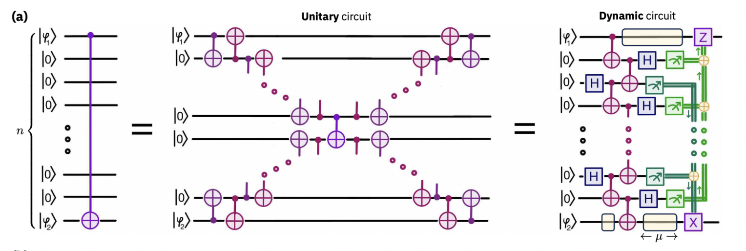
Wie im Bild zeigt, lauft de Prozess so:

1. Bereitstelle e Chetti vo Bell-Paar, wo d'Control- und Target-Qubits über Zwüscheancillas verbindet.
2. Füehrt Bell-Messige zwüsche nöd-verschränkte Nochberqubits dure, swappt Verschränkig Schritt för Schritt, bis Control und Target es Bell-Paar teiled.
3. Bruucht das Bell-Paar för Gate-Teleportation, wandlet es lokals CNOT i es deterministischs Langstrecke-CNOT i konstante Tiifi um.

De Aasatz ersetzt langi SWAP-Chetti mit em konstante Tiifi-Protokoll, reduziert d'Aafälligkeit för Zwoi-Qubit-Gatterfähler und macht d'Operation skalierbar mit de Gerätgröössi.

Im Folgende gönd mer zerscht dure d'dynamischi Schaltkreis-Implementierig vom LRCX-Schaltkreis. Am Änd stelle mer au e unitäri Implementierig för Vergliich vor, zum d'Vorteile vo dynamische Schaltkreis i däm Setting z'zeige.

(i) Schaltkreis initialisiere

Mer fanged mit em eifache Quante-Problem aa, wo als Basis för Vergliich dienet. Konkret initialisiere mer es Schaltkreis mit em Control-Qubit bim Index 0 und leged es Hadamard-Gatter druf. Das produziert e Superpositions-Zuestand, wo, wenn em Controlled-X-Operation folgt, e Bell-Zuestand $(|00\rangle + |11\rangle)/\sqrt{2}$ zwüsche Control- und Target-Qubits generiert.

Bi däm Punkt konstruiere mer no nöd s'Langstrecke-Controlled-X (LRCX) selber. Stattdesse isch euses Ziil, e chlarä und minimalä Aafangsschaltkreis z'definiere, wo d'Rolle vom LRCX ufzeigt. Im Schritt 2 zeige mer, wie s'LRCX als Optimierig mit dynamische Schaltkreis implementiert werde chan und vergliche sini Performance gege es unitärs Äquivalent. Wichtig isch, dass s'LRCX-Protokoll uf jede Aafangsschaltkreis aagwendet werde chan. Da bruuche mer das eifachi Hadamard-Setup för chlari Demonstration.

distance = 6  # The distance of the CNOT gate, with the convention that a distance of zero is a nearest-neighbor CNOT.

def initialize_circuit(distance):
    assert distance >= 0
    control = 0  # control qubit
    n = distance  # number of qubits between target and control

    qr = QuantumRegister(
        n + 2, name="q"
    )  # Circuit with n qubits between control and target
    cr = ClassicalRegister(
        2, name="cr"
    )  # Classical register for measuring control and target qubits

    k = int(n / 2)  # Number of Bell States to be used

    allcr = [cr]
    if (
        distance > 1
    ):  # This classical register will be used to store ZZ measurements. It is only used for long-range CX gates with distance > 1
        c1 = ClassicalRegister(
            k, name="c1"
        )  # Classical register needed for post processing
        allcr.append(c1)
    if (
        distance > 0
    ):  # This classical register will be used to store XX measurements. It is only used if distance > 0
        c2 = ClassicalRegister(
            n - k, name="c2"
        )  # Classical register needed for post processing
        allcr.append(c2)

    qc = QuantumCircuit(qr, *allcr, name="CNOT")

    # Apply a Hadamard gate to the control qubit such that the long-range CNOT gate will prepare a Bell state (|00> + |11>)/sqrt(2)
    qc.h(control)

    return qc

qc = initialize_circuit(distance)
qc.draw(fold=-1, output="mpl", scale=0.5)

Schritt 2: Problem för Quantehardware-Uusfüehrig optimiere

I däm Schritt zeige mer, wie mer de LRCX-Schaltkreis mit dynamische Schaltkreis konstruiere. S'Ziil isch, de Schaltkreis för d'Uusfüehrig uf Hardware z'optimiere, indem mer d'Tiifi im Vergliich zu ere rein unitäre Implementierig reduziere. Zum d'Vorteile z'illustriere, zeige mer sowohl d'dynamischi LRCX-Konstruktion als au ihres unitärs Äquivalent und vergliche spöter ihri Performance nach de Transpilation. Wichtig isch, dass mer da s'LRCX uf es eifachs Hadamard-initialisiertes Problem aawende, s'Protokoll chan aber uf jede Schaltkreis aagwendet werde, wo es Langstrecke-CNOT nötig isch.

(ii) Bell-Paar vorbereite

Mer fanged demit aa, e Chetti vo Bell-Paar längs em Pfad zwüsche Control- und Target-Qubits z'erstelle. Falls d'Distanz ungradi isch, wende mer zerscht es CNOT vom Control zu sim Nochber aa, das isch s'CNOT, wo teleportiert wird. För e gradi Distanz wird das CNOT nach em Bell-Paar-Vorbereite-Schritt aagwendet. S'Bell-Paar-Chetti verschränkt dänn nonenand ligendi Qubit-Paar und etabliert d'Ressuure, wo bruucht wird, zum d'Control-Information über s'Gerät z'träge.

# Determine where to start the Bell pair chain and add an extra CNOT when n is odd
def check_even(n: int) -> int:
    """Return 1 if n is even, else 2."""
    return 1 if n % 2 == 0 else 2

def prepare_bell_pairs(qc, add_barriers=True):
    n = qc.num_qubits - 2  # number of qubits between target and control
    k = int(n / 2)

    if add_barriers:
        qc.barrier()

    x0 = check_even(n)
    if n % 2 != 0:
        qc.cx(0, 1)

    # Create k Bell pairs
    for i in range(k):
        qc.h(x0 + 2 * i)
        qc.cx(x0 + 2 * i, x0 + 2 * i + 1)
    return qc

qc = prepare_bell_pairs(qc)
qc.draw(output="mpl", fold=-1, scale=0.5)

(iii) Nochberqubit-Paar i de Bell-Basis mässe

Als nöchsts mässe mer nöd-verschränkti Nochberqubits i de Bell-Basis (Zwoi-Qubit-Messige vo $XX$ und $ZZ$). Das chreiert es Langstrecke-Bell-Paar zwüsche em Target-Qubit und em Qubit näbe em Control (bis uf Pauli-Korrekture, wo über Feedforward im nöchste Schritt implementiert werded). Parallel dezu implementiere mer d'verschränkendi Messig, wo s'CNOT-Gatter teleportiert, zum uf s'beabsichtigte Target-Qubit z'wirke.

def measure_bell_basis(qc, add_barriers=True):
    n = qc.num_qubits - 2  # number of qubits between target and control
    k = int(n / 2)

    if n > 1:
        _, c1, c2 = qc.cregs
    elif n > 0:
        _, c2 = qc.cregs

    # Determine where to start the Bell pair chain and add an extra CNOT when n is odd
    x0 = 1 if n % 2 == 0 else 2

    # Entangling layer that implements the Bell measurement (and additionally adds the CNOT to be teleported, if n is even)
    for i in range(k + 1):
        qc.cx(x0 - 1 + 2 * i, x0 + 2 * i)

    for i in range(1, k + x0):
        if i == 1:
            qc.h(2 * i + 1 - x0)
        else:
            qc.h(2 * i + 1 - x0)

    if add_barriers:
        qc.barrier()

    # Map the ZZ measurements onto classical register c1
    for i in range(k):
        if i == 0:
            qc.measure(2 * i + x0, c1[i])
        else:
            qc.measure(2 * i + x0, c1[i])

    # Map the XX measurements onto classical register c2
    for i in range(1, k + x0):
        if i == 1:
            qc.measure(2 * i + 1 - x0, c2[i - 1])
        else:
            qc.measure(2 * i + 1 - x0, c2[i - 1])
    return qc

qc = measure_bell_basis(qc)
qc.draw(output="mpl", fold=-1, scale=0.5)

(iv) Als nöchsts Feedforward-Korrekture aawende, zum Pauli-Byprodukt-Operatore z'korrigiere

D'Bell-Basis-Messige füehred Pauli-Byprodukti ii, wo mit de ufgnommene Resultat korrigiert werde müend. Das gseht i zwoi Schritt. Zerscht müemer d'Parität vo allne $ZZ$-Messige berechne, wo dänn bruucht wird, zum bedingt es $X$-Gatter ufs Target-Qubit aazwende. Gliichso wird d'Parität vo de $XX$-Messige berechnet und bruucht, zum bedingt es $Z$-Gatter ufs Control-Qubit aazwende.

Mit em neue klassische Expression-Framework i Qiskit chönd die Paritäte direkt i de klassische Verarbeitigs-Schicht vom Schaltkreis berechnet werde. Aastatt e Reihefolgä vo einzelne bedingte Gatter för jedes Messigs-Bit aazwende, chönd mer e einzelni klassischi Expression baue, wo s'XOR (Parität) vo allne relevante Messigs-Resultat darstellt. Die Expression wird dänn als Bedingig i em einzelne if_test-Block bruucht, was es de Korrektur-Gatter erlaubt, i konstante Tiifi aagwendet z'werde. De Aasatz vereinfacht sowohl de Schaltkreis als au stellet sicher, dass d'Feedforward-Korrekture kei unnötigi zuesätzlichi Latenz iifüehred.

def apply_ffwd_corrections(qc):
    control = 0  # control qubit
    target = qc.num_qubits - 1  # target qubit
    n = qc.num_qubits - 2  # number of qubits between target and control

    k = int(n / 2)
    x0 = check_even(n)

    if n > 1:
        _, c1, c2 = qc.cregs
    elif n > 0:
        _, c2 = qc.cregs

    # First, let's compute the parity of all ZZ measurements
    for i in range(k):
        if i == 0:
            parity_ZZ = expr.lift(
                c1[i]
            )  # Store the value of the first ZZ measurement in parity_ZZ
        else:
            parity_ZZ = expr.bit_xor(
                c1[i], parity_ZZ
            )  # Successively compute the parity via XOR operations

    for i in range(1, k + x0):
        if i == 1:
            parity_XX = expr.lift(
                c2[i - 1]
            )  # Store the value of the first XX measurement in parity_XX
        else:
            parity_XX = expr.bit_xor(
                c2[i - 1], parity_XX
            )  # Successively compute the parity via XOR operations

    if n > 0:
        with qc.if_test(parity_XX):
            qc.z(control)

    if n > 1:
        with qc.if_test(parity_ZZ):
            qc.x(target)
    return qc

qc = apply_ffwd_corrections(qc)
qc.draw(output="mpl", fold=-1, scale=0.5)

(v) Zum Schluss Control- und Target-Qubits mässe

Mer definiere e Helper-Funktion, wo s'möglich macht, Control- und Target-Qubits i de $XX$-, $YY$- oder $ZZ$-Base z'mässe. För d'Verifizierig vom Bell-Zuestand $(|00\rangle + |11\rangle)/\sqrt{2}$ sötted d'Erwartigs wärt vo $XX$ und $ZZ$ beidi $+1$ sii, will si Stabilisatore vom Zuestand sind. D' $YY$-Messig wird da au understützt und wird unde bruucht, wenn mer d'Fidelity berechned.

def measure_in_basis(qc, basis="XX", add_barrier=True):
    control = 0  # control qubit
    target = qc.num_qubits - 1  # target qubit

    assert basis in ["XX", "YY", "ZZ"]

    qc = (
        qc.copy()
    )  # We copy the circuit because we want to measure in different bases
    cr = qc.cregs[0]

    if add_barrier:
        qc.barrier()

    if basis == "XX":
        qc.h(control)
        qc.h(target)
    elif basis == "YY":
        qc.sdg(control)
        qc.sdg(target)
        qc.h(control)
        qc.h(target)

    qc.measure(control, cr[0])
    qc.measure(target, cr[1])
    return qc

qc_YY = measure_in_basis(qc.copy(), basis="YY")
display(
    qc_YY.draw(output="mpl", fold=-1, scale=0.5)
)  # Circuit for measuring in the YY basis

S'ganze zämmesetze

Mer kombiniere d'verschidene Schritt vo obe, zum es Langstrecke-CX-Gatter uf zwei Ände vo ere 1D-Linie z'kreiere. D'Schritt sind

• S'Control-Qubit i $\\ket{+}$ initialisiere
• Bell-Paar vorbereite
• Nochberqubit-Paar mässe
• Feedforward-Korrekture abhängig vo de MCMs aawende

def lrcx(distance, prep_barrier=True, pre_measure_barrier=True):
    qc = initialize_circuit(distance)
    qc = prepare_bell_pairs(qc, prep_barrier)
    qc = measure_bell_basis(qc, pre_measure_barrier)
    qc = apply_ffwd_corrections(qc)
    return qc

qc = lrcx(distance)
# Apply the measurement in the XX, YY, and ZZ bases
qc_XX, qc_YY, qc_ZZ = [
    measure_in_basis(qc, basis=basis) for basis in ["XX", "YY", "ZZ"]
]

display(
    qc_YY.draw(output="mpl", fold=-1, scale=0.5)
)  # Circuit for measuring in the YY basis

Schaltkreis för verschideni Distanze generiere

Mer generiere jetz Langstrecke-CX-Schaltkreis för e Beriich vo Qubit-Trennige. För jedi Distanz baue mer Schaltkreis, wo i de $XX$-, $YY$- und $ZZ$-Base mässed, wo spöter bruucht werded, zum Fidelitys z'berechne.

D'Lischt vo Distanze enthält sowohl churzi als au langi Trennige, wobei distance = 0 em nöchsti-Nochber-CX entspricht. Die gliiche Distanze werded au spöter bruucht, zum di entsprechende unitäre Schaltkreis för Vergliich z'generiere.

distances = [
    0,
    1,
    2,
    3,
    6,
    11,
    16,
    21,
    28,
    35,
    44,
    55,
    60,
]  # Distances for long range CX. distance of 0 is a nearest-neighbor CX
distances.sort()
assert (
    min(distances) >= 0
)  # Only works for distance larger than 2 because classical register cannot be empty
basis_list = ["XX", "YY", "ZZ"]

circuits_dyn = []
for distance in distances:
    for basis in basis_list:
        circuits_dyn.append(
            measure_in_basis(lrcx(distance, prep_barrier=False), basis=basis)
        )
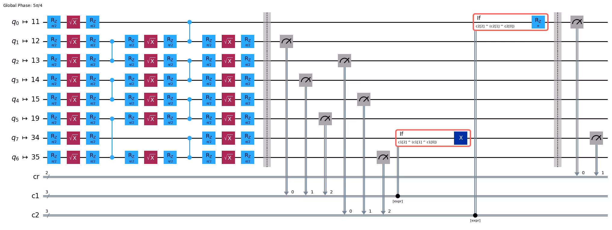
print(f"Number of circuits: {len(circuits_dyn)}")
circuits_dyn[14].draw(fold=-1, output="mpl", idle_wires=False)

Number of circuits: 39

Unitäri Implementierig, wo d'Qubits i d'Mitti swappt

För Vergliich undersueche mer zerscht de Fall, wo es Langstrecke-CNOT-Gatter mit nöchsti-Nochber-Verbindige und unitäre Gatter implementiert wird. Im folgende Bild isch links es Schaltkreis för es Langstrecke-CNOT-Gatter, wo e 1D-Chetti vo n-Qubits überspannt, wobei nume nöchsti-Nochber-Verbindige bruucht werded. I de Mitti isch e äquivalenti unitäri Zerlägig, wo mit lokale CNOT-Gatter implementierbar isch, Schaltkreistiifi $O(n)$.

De Schaltkreis i de Mitti chan so implementiert werde:

def cnot_unitary(distance):
    """Generate a long range CNOT gate using local CNOTs on a 1D chain of qubits subject to n
    nearest-neighbor connections only.

    Args:
        distance (int) : The distance of the CNOT gate, with the convention that a distance of 0 is a nearest-neighbor CNOT.

    Returns:
        QuantumCircuit: A Quantum Circuit implementing a long-range CNOT gate between qubit 0 and qubit distance+1
    """
    assert distance >= 0
    n = distance  # number of qubits between target and control

    qr = QuantumRegister(
        n + 2, name="q"
    )  # Circuit with n qubits between control and target
    cr = ClassicalRegister(
        2, name="cr"
    )  # Classical register for measuring control and target qubits

    qc = QuantumCircuit(qr, cr, name="CNOT_unitary")

    control_qubit = 0

    qc.h(control_qubit)  # Prepare the control qubit in the |+> state

    k = int(n / 2)
    qc.barrier()
    for i in range(control_qubit, control_qubit + k):
        qc.cx(i, i + 1)
        qc.cx(i + 1, i)
        qc.cx(-i - 1, -i - 2)
        qc.cx(-i - 2, -i - 1)
    if n % 2 == 1:
        qc.cx(k + 2, k + 1)
        qc.cx(k + 1, k + 2)
    qc.barrier()
    qc.cx(k, k + 1)
    for i in range(control_qubit, control_qubit + k):
        qc.cx(k - i, k - 1 - i)
        qc.cx(k - 1 - i, k - i)
        qc.cx(k + i + 1, k + i + 2)
        qc.cx(k + i + 2, k + i + 1)
    if n % 2 == 1:
        qc.cx(-2, -1)
        qc.cx(-1, -2)

    return qc

Jetz baue mer alli unitäre Schaltkreis und erstelle d'Schaltkreis, wo i de $XX$-, $YY$- und $ZZ$-Base mässed, gliich wie mer's för d'dynamische Schaltkreis obe gmacht händ.

circuits_uni = []
for distance in distances:
    for basis in basis_list:
        circuits_uni.append(
            measure_in_basis(cnot_unitary(distance), basis=basis)
        )

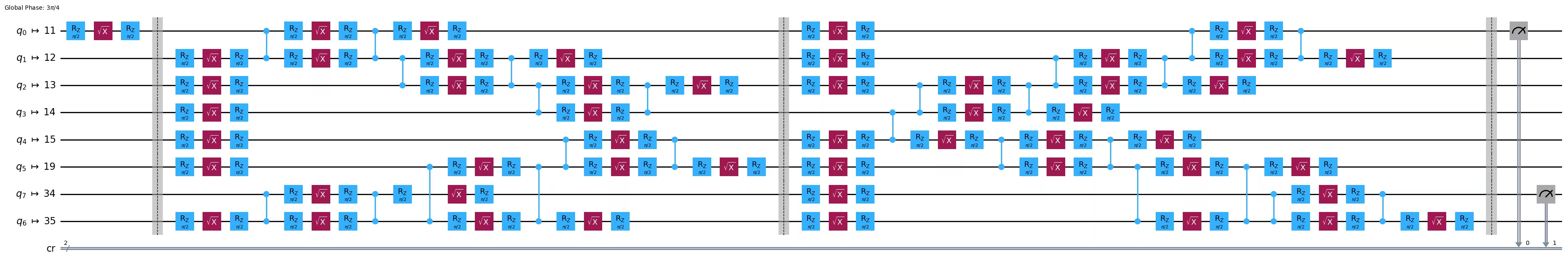
print(f"Number of circuits: {len(circuits_uni)}")
circuits_uni[14].draw(fold=-1, output="mpl", idle_wires=False)

Number of circuits: 39

Jetz, wo mer sowohl dynamischi als au unitäri Schaltkreis för e Beriich vo Distanze händ, sind mer parat för Transpilation. Mer müend zerscht es Backend-Gerät uuswähle.

# Set up access to IBM Quantum devices
from qiskit.circuit import IfElseOp

service = QiskitRuntimeService()
backend = service.least_busy(
    operational=True, simulator=False, min_num_qubits=156
)

De folgend Schritt stellet sicher, dass s'Backend d' if_else-Instrukzioon understützt, wo för d'neueri Version vo dynamische Schaltkreis bruucht wird. Will die Funkzioon no im Early Access isch, füeged mer s' IfElseOp explizit zum Backend-Target dezue, falls es no nöd verfüegbar isch.

if "if_else" not in backend.target.operation_names:
    backend.target.add_instruction(IfElseOp, name="if_else")

Layer Fidelity String för Uuswahl vo ere 1D-Chetti bruuche

Will mer d'Performance vo dynamische und unitäre Schaltkreis uf ere 1D-Chetti vergliche wänd, bruuche mer de Layer Fidelity String, zum e lineari Topologie vo de beste Chetti vo Qubits usem Gerät uuszwähle. Das stellet sicher, dass beidi Arte vo Schaltkreis under de gliiche Konnektivitäts-Iischränkige transpiliert werded, was e faire Vergliich vo ihre Performance erlaubt.

# This selects best qubits for longest distance and uses the same control for all lengths
lf_qubits = backend.properties().to_dict()[
    "general_qlists"
]  # best linear chain qubits
chosen_layouts = {
    distance: [
        val["qubits"]
        for val in lf_qubits
        if val["name"] == f"lf_{distances[-1] + 2}"
    ][0][: distance + 2]
    for distance in distances
}
print(chosen_layouts[max(distances)])  # best qubits at each distance

[10, 11, 12, 13, 14, 15, 19, 35, 34, 33, 39, 53, 54, 55, 59, 75, 74, 73, 72, 71, 58, 51, 50, 49, 48, 47, 46, 45, 44, 43, 56, 63, 62, 61, 76, 81, 82, 83, 84, 85, 77, 65, 66, 67, 68, 69, 78, 89, 90, 91, 98, 111, 110, 109, 108, 107, 106, 105, 104, 103, 102, 101]

isa_circuits_dyn = []
isa_circuits_uni = []

# Using the same initial layouts for both circuits for better apples to apples comparison
for qc in circuits_dyn:
    pm = generate_preset_pass_manager(
        optimization_level=1,
        backend=backend,
        initial_layout=chosen_layouts[qc.num_qubits - 2],
    )
    isa_circuits_dyn.append(pm.run(qc))

for qc in circuits_uni:
    pm = generate_preset_pass_manager(
        optimization_level=1,
        backend=backend,
        initial_layout=chosen_layouts[qc.num_qubits - 2],
    )
    isa_circuits_uni.append(pm.run(qc))

print(
    f"2Q depth: {isa_circuits_dyn[14].depth(lambda x: x.operation.num_qubits == 2)}"
)
isa_circuits_dyn[14].draw("mpl", fold=-1, idle_wires=0)

2Q depth: 2

print(
    f"2Q depth: {isa_circuits_uni[14].depth(lambda x: x.operation.num_qubits == 2)}"
)
isa_circuits_uni[14].draw("mpl", fold=-1, idle_wires=False)

2Q depth: 13

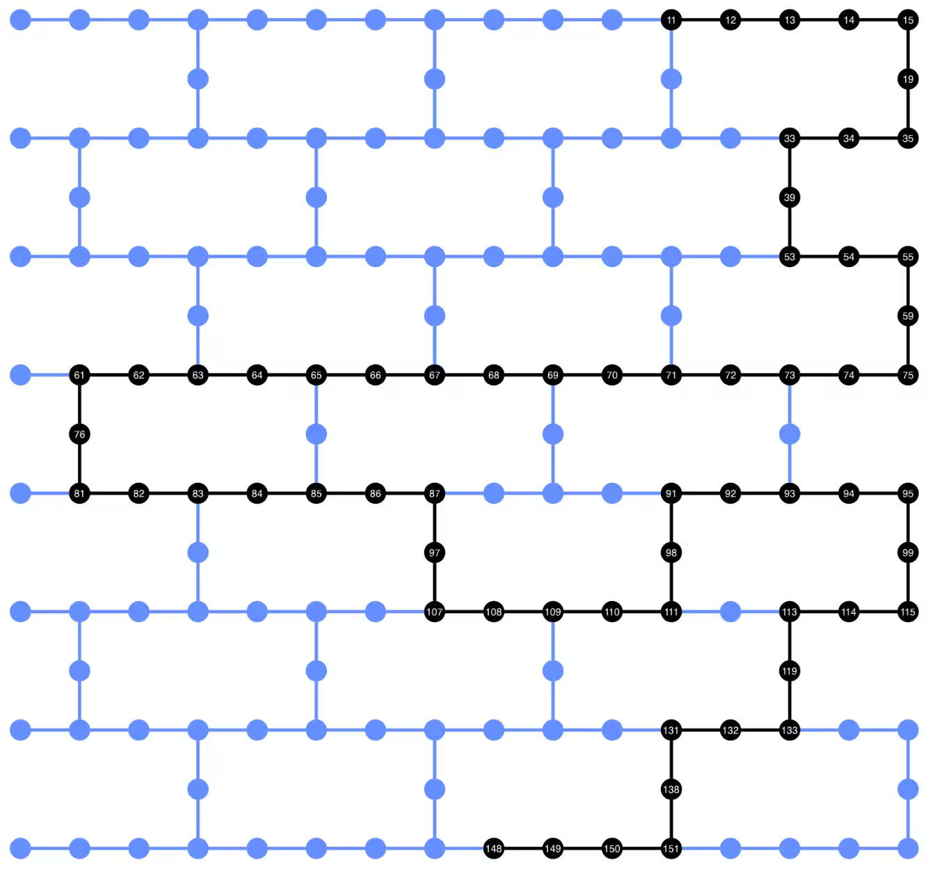
Visualisiered d Qubits wo für de LRCX-Schaltkreis bruucht werdet

I dem Abschnitt luege mer aa, wie de LRCX-Schaltkreis uf d Hardware abbildet wird. Mer fanget aa mit de Visualisierig vo de physische Qubits wo im Schaltkreis bruucht werdet und undersueched denn, wie de Control-Target-Abschtand im Layout d Azahl vo Operatione beyflusst.

# Note: the qubit coordinates must be hard-coded.
# The backend API does not currently provide this information directly.
# If using a different backend, you will need to adjust the coordinates accordingly,
# or set the qubit_coordinates = None to use the default layout coordinates.

def _heron_coords_r2():
    """Generate coordinates for the Heron layout in R2. Note"""
    cord_map = np.array(
        [
            [
                0,
                1,
                2,
                3,
                4,
                5,
                6,
                7,
                8,
                9,
                10,
                11,
                12,
                13,
                14,
                15,
                3,
                7,
                11,
                15,
                0,
                1,
                2,
                3,
                4,
                5,
                6,
                7,
                8,
                9,
                10,
                11,
                12,
                13,
                14,
                15,
                1,
                5,
                9,
                13,
                0,
                1,
                2,
                3,
                4,
                5,
                6,
                7,
                8,
                9,
                10,
                11,
                12,
                13,
                14,
                15,
                3,
                7,
                11,
                15,
                0,
                1,
                2,
                3,
                4,
                5,
                6,
                7,
                8,
                9,
                10,
                11,
                12,
                13,
                14,
                15,
                1,
                5,
                9,
                13,
                0,
                1,
                2,
                3,
                4,
                5,
                6,
                7,
                8,
                9,
                10,
                11,
                12,
                13,
                14,
                15,
                3,
                7,
                11,
                15,
                0,
                1,
                2,
                3,
                4,
                5,
                6,
                7,
                8,
                9,
                10,
                11,
                12,
                13,
                14,
                15,
                1,
                5,
                9,
                13,
                0,
                1,
                2,
                3,
                4,
                5,
                6,
                7,
                8,
                9,
                10,
                11,
                12,
                13,
                14,
                15,
                3,
                7,
                11,
                15,
                0,
                1,
                2,
                3,
                4,
                5,
                6,
                7,
                8,
                9,
                10,
                11,
                12,
                13,
                14,
                15,
            ],
            -1
            * np.array([j for i in range(15) for j in [i] * [16, 4][i % 2]]),
        ],
        dtype=int,
    )

    hcords = []
    ycords = cord_map[0]
    xcords = cord_map[1]
    for i in range(156):
        hcords.append([xcords[i] + 1, np.abs(ycords[i]) + 1])

    return hcords

# Visualize the active qubits in the circuit layout
plot_circuit_layout(
    circuit=isa_circuits_uni[-1],
    backend=backend,
    view="physical",
    qubit_coordinates=_heron_coords_r2(),
)

Schritt 3: Usfüehrig mit Qiskit Primitives

I dem Schritt füehre mer s Experiment uf em spezifizierte Backend us. Mer nutze au Batching zum s Experiment effizient über meh Trials z laufe. Wiederholti Trials erlaube eus, Durchschnittswärt z berächne für e gnauere Vergliich zwüsche de unitäre und dynamische Methode, und au d Variabilität z quantifiziere dur de Vergliich vo de Abwychige über d Trials.

print(backend.name)

ibm_kingston

Wähled d Azahl vo Trials und füehred d Batch-Usfüehrig durch.

num_trials = 10
jobs_uni = []
jobs_dyn = []
with Batch(backend=backend) as batch:
    sampler = Sampler(mode=batch)
    for _ in range(num_trials):
        jobs_uni.append(sampler.run(isa_circuits_uni, shots=1024))
        jobs_dyn.append(sampler.run(isa_circuits_dyn, shots=1024))

Schritt 4: Nachbearbeitig und Rückgab vom Resultat im gwünschte klassische Format

Nachdem d Experiment erfolgriich usgfüehrt worde sind, verarbeite mer jetzt d Messresultat zum sinnvolli Metrike z extrahiere. I dem Schritt:

• Definiere mer Qualitätsmetrike zum Evaluiere vo de Leischtig vom Langstrecke-CX.
• Berächne mer Erwaartigswärt vo Pauli-Operatore us de roh Messresultat.
• Bruuche die zum d Fidelity vom generierte Bell-Zustand z berächne.

Die Analyse git es klars Bild, wie guet d dynamische Schaltkreis im Vergliich zur unitäre Baseline-Implementierig abschniidet.

Qualitätsmetrike

Zum de Erfolg vom Langstrecke-CX-Protokoll z evaluiere, messe mer wie nöch de Output-Zustand am ideale Bell-Zustand isch. E praktischi Art zum das z quantifiziere isch d Berächnig vo de State Fidelity über Erwaartigswärt vo Pauli-Operatore. D Fidelity für e Bell-Zustand uf em Control- und Target-Zustand chan berächnet werde nachdem mer $\braket{XX}$, $\braket{YY}$ und $\braket{ZZ}$ kännt. Im Speziälle:

$F = \frac{1}{4} (1 + \braket{XX} - \braket{YY} + \braket{ZZ})$

Zum die Erwaartigswärt us de roh Messdatene z berächne, definiere mer e Satz vo Hilfsfunktione:

• compute_ZZ_expectation: Git d Erwaartigswärt vo eme Zwoi-Qubit-Pauli-Operator i de $Z$-Basis zrugg, basierend uf de Messzähler.
• compute_fidelity: Kombiniert d Erwaartigswärt vo $XX$, $YY$ und $ZZ$ i de Fidelity-Formel obe.
• get_counts_from_bitarray: Hilfsfunktion zum Zähler us de Backend-Resultat-Objekt z extrahiere.

def compute_ZZ_expectation(counts):
    total = sum(counts.values())
    expectation = 0
    for bitstring, count in counts.items():
        # Ensure bitstring is 2 bits
        z1 = (-1) ** (int(bitstring[-1]))
        z2 = (-1) ** (int(bitstring[-2]))
        expectation += z1 * z2 * count
    return expectation / total

def compute_fidelity(counts_xx, counts_yy, counts_zz):
    xx, yy, zz = [
        compute_ZZ_expectation(c) for c in [counts_xx, counts_yy, counts_zz]
    ]
    return 1 / 4 * (1 + xx - yy + zz)

Mer berächne d Fidelity für d dynamische Langstrecke-CX-Schaltkreis. Für jedi Distanz extrahiere mer d Messresultat i de $\braket{XX}$-, $\braket{YY}$- und $\braket{ZZ}$-Base. Die Resultat werdet mit de vorane definierte Hilfsfunktione kombiniert zum d Fidelity z berächne gemäss $F = \tfrac{1}{4} \big( 1 + \langle XX \rangle - \langle YY \rangle + \langle ZZ \rangle \big)$. Das git d beobachteti Fidelity vom dynamisch usgfüehrte Protokoll bi jeder Distanz.

fidelities_dyn = []

# loop over trials
for job in jobs_dyn:
    result_dyn = job.result()
    trial_fidelities = []
    # loop over all distances
    for ind, dist in enumerate(distances):
        counts_xx = result_dyn[ind * 3].data.cr.get_counts()
        counts_yy = result_dyn[ind * 3 + 1].data.cr.get_counts()
        counts_zz = result_dyn[ind * 3 + 2].data.cr.get_counts()
        trial_fidelities.append(
            compute_fidelity(counts_xx, counts_yy, counts_zz)
        )
    fidelities_dyn.append(trial_fidelities)
# average over trials for each distance
avg_fidelities_dyn = np.mean(fidelities_dyn, axis=0)
std_fidelities_dyn = np.std(fidelities_dyn, axis=0)

Jetzt berächne mer d Fidelity für d unitäre Langstrecke-CX-Schaltkreis, uf die gliich Art wie mir das für d dynamische Schaltkreis obe gmacht händ.

fidelities_uni = []

# loop over trials
for job in jobs_uni:
    result_uni = job.result()
    trial_fidelities = []
    # loop over all distances
    for ind, dist in enumerate(distances):
        counts_xx = result_uni[ind * 3].data.cr.get_counts()
        counts_yy = result_uni[ind * 3 + 1].data.cr.get_counts()
        counts_zz = result_uni[ind * 3 + 2].data.cr.get_counts()
        trial_fidelities.append(
            compute_fidelity(counts_xx, counts_yy, counts_zz)
        )
    fidelities_uni.append(trial_fidelities)
# average over trials for each distance
avg_fidelities_uni = np.mean(fidelities_uni, axis=0)
std_fidelities_uni = np.std(fidelities_uni, axis=0)

D Resultat plotte

Zum d Resultat visuell z würdige, plottet d Zelle unne die gschätzte Gate-Fidelities, gmässe bi verschidene Distanze zwüsche de verschränkte Qubits für die Methode.

fig, ax = plt.subplots()

# Unitary with error bars
ax.errorbar(
    distances,
    avg_fidelities_uni,
    yerr=std_fidelities_uni,
    fmt="o-.",
    color="c",
    ecolor="c",
    elinewidth=1,
    capsize=4,
    label="Unitary",
)
# Dynamic with error bars
ax.errorbar(
    distances,
    avg_fidelities_dyn,
    yerr=std_fidelities_dyn,
    fmt="o-.",
    color="m",
    ecolor="m",
    elinewidth=1,
    capsize=4,
    label="Dynamic",
)
# Random gate baseline
ax.axhline(y=1 / 4, linestyle="--", color="gray", label="Random gate")

legend = ax.legend(frameon=True)
for text in legend.get_texts():
    text.set_color("black")
legend.get_frame().set_facecolor("white")
legend.get_frame().set_edgecolor("black")
ax.set_title(
    "Bell State Fidelity vs Control–Target Separation", color="black"
)
ax.set_xlabel("Distance", color="black")
ax.set_ylabel("Bell state fidelity", color="black")
ax.grid(linestyle=":", linewidth=0.6, alpha=0.4, color="gray")
ax.set_ylim((0.2, 1))
ax.set_facecolor("white")
fig.patch.set_facecolor("white")
for spine in ax.spines.values():
    spine.set_visible(True)
    spine.set_color("black")
ax.tick_params(axis="x", colors="black")
ax.tick_params(axis="y", colors="black")
plt.show()

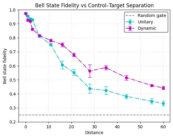
Us em Fidelity-Plot obe het de LRCX nöd konsistent besser abgschnitte als d direkt unitäri Implementierig. Tatsächlich het de unitäri Schaltkreis bi churze Control-Target-Abschtänd e höcheri Fidelity erreicht. Allerdings fangt de dynamisch Schaltkreis bi grössere Abschtänd aa, e besseri Fidelity als d unitäri Implementierig z erreiche. Das Verhalte isch uf de aktuälle Hardware nöd unerwartet: Während dynamischi Schaltkreis d Schaltkreistiifi reduziere dur s Vermiide vo lange SWAP-Chetti, füehre si zuesätzlichi Schaltkreiszyt y dur Mid-Circuit-Messige, klassischs Feedforward und Control-Path-Verzögerige. D zuesätzlich Latänz erhöht d Decoheränz und Uslesefähler, was bi churze Distanze d Tiifeneinsparige überwoge chan.

Trotzdem beobachte mer e Chrüzigspunkt, wo de dynamisch Aasatz de unitär überholt. Das isch es direkts Resultat vo de unterschidliche Skalierig: D Tiifi vom unitäre Schaltkreis wachst linear mit de Distanz zwüsche de Qubits, während d Tiifi vom dynamische Schaltkreis konstant bliibt.

Schlüsselpünkt:

• Sofortige Vorteil vo dynamische Schaltkreis: D Hauptmotivation hüt isch d reduzierted Zwoi-Qubit-Tiifi, nöd zwingend e verbesserted Fidelity.
• Warum d Fidelity hüt schlächter sy chan: Erhöhti Schaltkreiszyt dur Messig- und klassischi Operatione dominiere oft, bsunders wenn de Control-Target-Abschtand chly isch.
• Usblick: Wenn d Hardware sich verbesseret, speziell schnälleri Uslesig, chürzeri klassischi Kontrolllatänz und reduzierte Mid-Circuit-Overhead, sötte mer erwarte, dass die Tiife- und Duurreduktione sich i messbare Fidelity-Gwinne übersetze.

# Compute metrics for each distance, skipping the basis circuits since they are identical for each distance
depths_2q_dyn = [
    c.depth(lambda x: x.operation.num_qubits == 2)
    for c in isa_circuits_dyn[::3]
]
meas_dyn = [
    sum(1 for instr in c.data if instr.operation.name == "measure")
    for c in isa_circuits_dyn[::3]
]

depths_2q_uni = [
    c.depth(lambda x: x.operation.num_qubits == 2)
    for c in isa_circuits_uni[::3]
]
meas_uni = [
    sum(1 for instr in c.data if instr.operation.name == "measure")
    for c in isa_circuits_uni[::3]
]

fig, axes = plt.subplots(1, 2, figsize=(12, 5))

axes[0].plot(
    distances, depths_2q_uni, "o-.", color="c", label="Unitary (2Q depth)"
)
axes[0].plot(
    distances, depths_2q_dyn, "o-.", color="m", label="Dynamic (2Q depth)"
)
axes[0].set_xlabel("Number of qubits between control and target")
axes[0].set_ylabel("Two-qubit depth")
axes[0].grid(True, linestyle=":", linewidth=0.6, alpha=0.4)
axes[0].legend()

axes[1].plot(
    distances, meas_uni, "o-.", color="c", label="Unitary (# measurements)"
)
axes[1].plot(
    distances, meas_dyn, "o-.", color="m", label="Dynamic (# measurements)"
)
axes[1].set_xlabel("Number of qubits between control and target")
axes[1].set_ylabel("Number of measurements")
axes[1].grid(True, linestyle=":", linewidth=0.6, alpha=0.4)
axes[1].legend()

fig.suptitle("Scaling of Unitary vs Dynamic LRCX with Distance", fontsize=12)

plt.tight_layout()
plt.show()

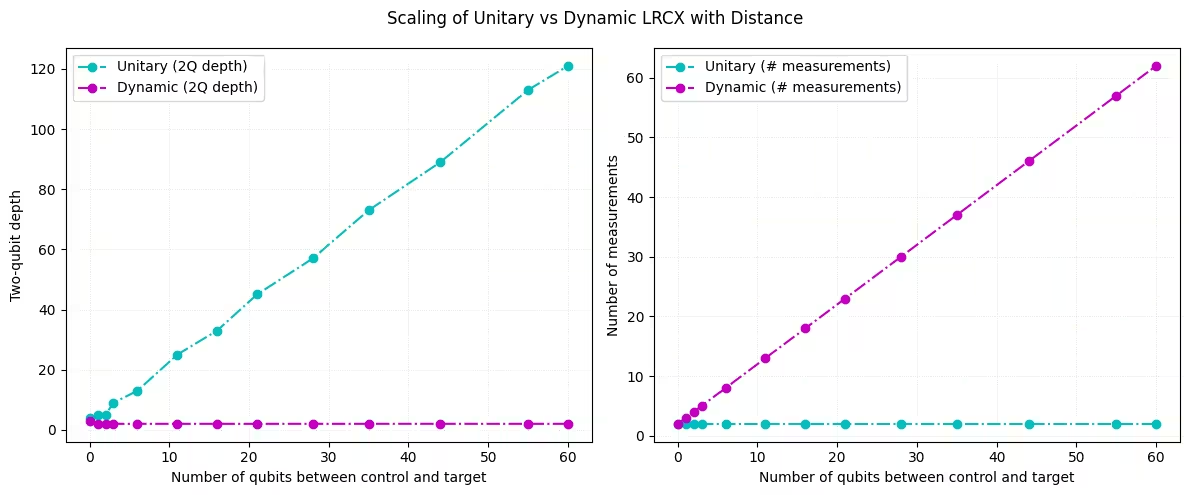
De Zwoi-Qubit-Tiife-Plot zeigt de Hauptvorteil vom LRCX wo mit dynamische Schaltkreis implementiert isch: D Performance bliibt im Wesentliche konstant wenn de Abschtand zwüsche Control- und Target-Qubits zunimmt. Im Gegesatz dezue wachst d unitäri Implementierig linear mit de Distanz wäge de nötige SWAP-Chetti. D Tiifi erfasst d logischi Skalierig vo Zwoi-Qubit-Operatione, während d Messazahl de zuesätzlich Overhead für dynamischi Schaltkreis widerspieglet. Die Messige sind effizient, da si parallel usgfüehrt werdet, aber si füehre uf de hütige Hardware trotzdem festi Choschte y.

Warum d Fidelity hüt schlächter sy chan: Erhöhti Schaltkreiszyt dur Messig- und klassischi Operatione dominiere oft, bsunders wenn de Control-Target-Abschtand chly isch. Zum Bispil isch d durchschnittlich Usleselängi uf emene Heron r2-Prozessor 2'280 ns, während d 2Q-Gatterlängi nur 68 ns isch.

Wenn d Messig- und klassischi Latänze sich verbessere, erwarte mer, dass d konstant-tiifi und konstant-Messig-Skalierig vo dynamische Schaltkreis klari Fidelity- und Laufzyt-Vorteil bi grössere Schaltkreis bringt.

Referänze

[1] Efficient Long-Range Entanglement using Dynamic Circuits, by Elisa Bäumer, Vinay Tripathi, Derek S. Wang, Patrick Rall, Edward H. Chen, Swarnadeep Majumder, Alireza Seif, Zlatko K. Minev. IBM Quantum, (2023). https://arxiv.org/abs/2308.13065