Nonig übersetzt

Di Siite isch nonig übersetzt worde. Dir luege d englischi Originalversion aa.

QUICK-PDE: A Qiskit Function by ColibriTD

hinwiis

Qiskit Functions are an experimental feature available to IBM Quantum® Premium Plan, Flex Plan, and On-Prem (via IBM Quantum Platform API) Plan users. They are in preview release status and subject to change.

Overview

The Partial Differential Equation (PDE) solver presented here is part of our Quantum Innovative Computing Kit (QUICK) platform (QUICK-PDE), and is packaged as a Qiskit Function. With the QUICK-PDE function, you can solve domain-specific partial differential equations on IBM Quantum QPUs. This function is based on the algorithm described in ColibriTD's H-DES description paper. This algorithm can solve complex multi-physics problems, starting with Computational Fluid Dynamics (CFD) and Materials Deformation (MD), and other use cases coming soon.

To tackle the differential equations, the trial solutions are encoded as linear combinations of orthogonal functions (typically Chebyshev polynomials, and more specifically $2^n$ of them where $n$ is the number of qubits encoding your function), parametrized by the angles of a Variable Quantum Circuit (VQC). The ansatz generates a state encoding the function, which is evaluated by observables whose combinations allow for evaluating the function at all points. You can then evaluate the loss function in which the differential equations are encoded, and fine-tune the angles in a hybrid loop, as shown in the following. The trial solutions get gradually closer to the actual solutions until you reach a satisfactory result.

In addition to this hybrid loop, you can also chain together different optimizers. This is useful when you want a global optimizer to find a good set of angles, and then a more fine-tuned optimizer to follow a gradient to the best set of neighboring angles. In the case of computational fluid dynamics (CFD), the default optimization sequence produces the best results - but in the case of material deformation (MD), while the default provides good results, you can configure it further for problem-specific benefits.

Note for each variable of the function, we specify number of qubits (which you can play with). By stacking 10 identical circuits and evaluating the 10 identical observables on different qubits throughout one big circuit, you can noise-mitigate within the CMA optimization process, relying on the noise learner method, and significantly reduce the number of shots needed.

Input/output

Computational Fluid Dynamics

The inviscid Burgers' equation, models flowing non-viscous fluids as follows:

$\frac{\partial u}{\partial t} + u\frac{\partial u}{\partial x} = 0,$

$u$ represents the fluid speed field. This use-case has a temporal boundary condition: you can select the initial condition and then allow the system to relax. Currently, the only accepted initial conditions are linear functions: $ax + b$.

The arguments for CFD's differential equations are on a fixed grid, as follows:

• $t$ is between 0 and 0.95 with 30 sample points. $x$ is between 0 and 0.95 with a step size of 0.2375.

Material Deformation

This use case focuses on hypoelastic deformation with the one-dimensional tensile test, in which a bar fixed in space is pulled at its other extremity. We describe the problem as follows:

$u' - \frac{\sigma}{3K} - \frac{2}{\sqrt{3}}\epsilon_0\left(\frac{\sigma'}{\sigma_0\sqrt{3}}\right)^n = 0$

$\sigma' - b = 0,$

$K$ represents the bulk modulus of the material being stretched, $n$ the exponent of a power law, $b$ the force per unit mass, $\epsilon_0$ the proportional stress limit, $\sigma_0$ the proportional strain limit, $u$ the stress function, and $\sigma$ the strain function.

The considered bar is of unitary length. This use-case has a boundary condition for surface stress $t$, or the amount of work needed to stretch the bar.

The arguments for MD's differential equations are on a fixed grid, as follows:

• $x$ is between 0 and 1 with a step size of 0.04.

Input

In order to run the QUICK-PDE Qiskit Function, you can adjust the following parameters:

Name	Type	Description	Use-case specific	Example
use_case	Literal["MD", "CFD"]	Toggle to select the system of differential equations to solve	No	"CFD"
parameters	dict[str, Any]	Parameters of the differential equation (see the next table for more detail)	No	{"a": 1.0, "b": 1.0}
nb_qubits	Optional[dict[str, dict[str, int]]]	Number of qubits per function and per variable. Optimized values are chosen by the function, but if you want to try to find a better combination, you can override the default values	No	{"u": {"x": 1, "t":3}}
depth	Optional[dict[str, int]]	Depth of ansatz per function. Optimized values are chosen by the function, but if you want to try to find a better combination, you can override the default values	No	{"u": 4}
optimizer	Optional[list[str]]	Optimizers to be used, either "CMAES" from the cma python library or one of the optimizers of scipy	MD	"SLSQP"
shots	Optional[list[int]]	Number of shots used to run each circuit. Since several optimization steps are needed, the length of the list must be equal to the number of optimizers used (4 in the case of CFD). Defaults to [50_000] * nb_optimizers for MD and [5_00, 2_000, 5_000, 10_000] for CFD	No	[15_000, 30_000]
optimizer_options	Optional[dict[str, Any]]	Options to pass to the optimizer. The details of this input depends on the optimizer used; for specifics, refer to the documentation of the optimizer used	MD	{"maxiter": 50 }
initialization	Optional[Literal["RANDOM", "PHYSICALLY_INFORMED"]]	Whether to start with random angles or smartly chosen angles. Beware that smartly chosen angles may not work in 100% of the cases. Defaults to "PHYSICALLY_INFORMED".	No	"RANDOM"
backend_name	Optional[str]	The backend name to use.	No	"ibm_torino"
mode	Optional[Literal["job", "session", "batch"]]	The execution mode to use. Defaults to "job".	No	"job"

The parameters of the differential equation (physical parameters and boundary condition) should follow the given format:

Use case	Key	Value type	Description	Example
CFD	a	float	Coefficient of the initial values of $u$	1.0
CFD	b	float	Offset of the initial values of $u$	1.0
MD	t	float	surface stress	12.0
MD	K	float	bulk modulus	100.0
MD	n	int	power law	4.0
MD	b	float	force per unit mass	10.0
MD	epsilon_0	float	proportional stress limit	0.1
MD	sigma_0	float	proportional strain limit	5.0

Output

The output is a dictionary with the list of sample points, as well as the values of the functions at each of these points:

# Added by doQumentation — required packages for this notebook
!pip install -q matplotlib numpy qiskit-ibm-catalog

from numpy import array

solution = {
    "functions": {
        "u": array(
            [
                [0.01, 0.1, 1],
                [0.02, 0.2, 2],
                [0.03, 0.3, 3],
                [0.04, 0.4, 4],
            ]
        ),
    },
    "samples": {
        "t": array([0.1, 0.2, 0.3, 0.4]),
        "x": array([0.5, 0.6, 0.7]),
    },
}

The shape of a solution array depends on the variables' samples:

assert len(solution["functions"]["u"].shape) == len(solution["samples"])
for col_size, samples in zip(
    solution["functions"]["u"].shape, solution["samples"].values()
):
    assert col_size == len(samples)

The mapping between the function variables' sample points and the solution array's dimension is done in alphanumeric order of the variable's name. For example, if the variables are "t" and "x", a row of solution["functions"]["u"] represents the values of the solution for a fixed "t", and a column of solution["functions"]["u"] represents the values of the solution for a fixed "x".

The following is an example of how to get the value of the function for a specific set of coordinate:

# u(t=0.2, x=0.7) == 2
assert solution["samples"]["t"][1] == 0.2
assert solution["samples"]["x"][2] == 0.7
assert solution["functions"]["u"][1, 2] == 2

Benchmarks

The following table presents statistics on various runs of our function.

Example	Number of qubits	Initialization	Error	Total time (min)	Runtime usage (min)
Inviscid Burgers' equation	50	PHYSICALLY_INFORMED	$10^{-2}$	66	25
Hypoelastic 1D tensile test	18	RANDOM	$10^{-2}$	123	100

Get started

Fill out the form to request access to the QUICK-PDE function. Then, assuming you've already saved your account to your local environment, select the function as follows:

from qiskit_ibm_catalog import QiskitFunctionsCatalog

catalog = QiskitFunctionsCatalog(channel="ibm_quantum_platform")

quick = catalog.load("colibritd/quick-pde")

Examples

To get started, try one of the following examples:

Computational Fluid Dynamics (CFD)

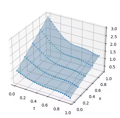
When initial conditions are set to $u(0,x) = x$, the results are as follows:

# launch the simulation with initial conditions u(0,x) = a*x + b
job = quick.run(use_case="cfd", physical_parameters={"a": 1.0, "b": 0.0})

Check your Qiskit Function workload's status or return results as follows:

print(job.status())
solution = job.result()

'QUEUED'

import numpy as np
import matplotlib.pyplot as plt

_ = plt.figure()
ax = plt.axes(projection="3d")

# plot the solution using the 3d plotting capabilities of pyplot
t, x = np.meshgrid(solution["samples"]["t"], solution["samples"]["x"])
ax.plot_surface(
    t,
    x,
    solution["functions"]["u"],
    edgecolor="royalblue",
    lw=0.25,
    rstride=26,
    cstride=26,
    alpha=0.3,
)
ax.scatter(t, x, solution["functions"]["u"], marker=".")
ax.set(xlabel="t", ylabel="x", zlabel="u(t,x)")

plt.show()

Material Deformation

The material deformation use case requires the physical parameters of your material and the applied force, as follows:

import matplotlib.pyplot as plt

# select the properties of your material
job = quick.run(
    use_case="md",
    physical_parameters={
        "t": 12.0,
        "K": 100.0,
        "n": 4.0,
        "b": 10.0,
        "epsilon_0": 0.1,
        "sigma_0": 5.0,
    },
)

# plot the result
solution = job.result()

_ = plt.figure()
stress_plot = plt.subplot(211)
plt.plot(solution["samples"]["x"], solution["functions"]["u"])
strain_plot = plt.subplot(212)
plt.plot(solution["samples"]["x"], solution["functions"]["sigma"])

plt.show()

Fetch error messages

If your workload status is ERROR, use job.error_message() to fetch the error message to help debug, as follows:

job = quick.run(use_case="mdf", physical_params={})

print(job.error_message())

# or write a wrapper around it for a more human readable version
def pprint_error(job):
    print("".join(eval(job.error_message())["error"]))

print("___")
pprint_error(job)

{"error": ["qiskit.exceptions.QiskitError: 'Unknown argument \"physical_params\", did you make a typo? -- https://docs.quantum.ibm.com/errors#1804'\n"]}
___
qiskit.exceptions.QiskitError: 'Unknown argument "physical_params", did you make a typo? -- https://docs.quantum.ibm.com/errors#1804'

Get support

For support, contact qiskit-function-support@colibritd.com.

Next steps

Recommendations

• Fill out the form to request access to the QUICK-PDE function.
• Try modeling a flowing non-viscous fluid using QUICK-PDE in the tutorial.
• Review Jaffali, H., et al. (2025). H-DES: a Quantum-Classical Hybrid Differential Equation Solver. arXiv preprint arXiv:2410.01130.